Sanity check: watch the time series before trusting the exponents

Before treating a Lyapunov-exponent estimate as meaningful, it’s worth first checking that the model behind step_fn is doing what you expect – settling onto the attractor you had in mind, not diverging, not stuck at a fixed point. step_fn (however it’s built – ode_problem, network_problem, …) is a plain state -> new_state map under the hood, so the exact function handed to lyapunov_spectrum can also just be run forward on its own and inspected as an ordinary time series – no separate simulation code path to maintain. lyapax.utils.simulate_trajectory( step_fn, state0, n_steps, dt=dt) does this: it iterates step_fn via jax.lax.scan and returns (t, traj), the matching time axis and the whole trajectory (shape (n_steps + 1, d), including the initial state). Both problem objects expose their built step_fn/state0 as plain attributes, so simulate_trajectory and lyapunov_spectrum can share the exact same problem without re-deriving anything.

Single system. The Lorenz system (also used in 03_chaotic_flows.py): the raw time series of x(t) should show the signature back-and-forth between the two lobes of the attractor, and z(t) should stay positive – both are quick visual checks that this is really behaving like the Lorenz attractor, not, say, diverging because of a sign error in the right-hand side.

Coupled network. The 4-node linear network from 04_linear_network.py: every eigenvalue of its Jacobian is negative, so every node’s time series should decay toward 0. A network step function built with network_problem has exactly the same state -> new_state shape as a plain ODE step, so simulate_trajectory needs no adapter to work with it.

Once the time series looks like what’s expected, lyapunov_spectrum is run on the same step_fn to get the exponents – “does the model behave as expected” and “what are its Lyapunov exponents” are two views of the same simulation, not two separate things to set up.

import os

os.environ["JAX_PLATFORMS"] = "cpu"

import jax
import jax.numpy as jnp
import matplotlib.pyplot as plt
import numpy as np

jax.config.update("jax_enable_x64", True)

from lyapax import systems
from lyapax.core import lyapunov_spectrum, ode_problem
from lyapax.coupling import linear_coupling
from lyapax.network import Network, network_problem
from lyapax.simulator import ModelSpec, Parameter, StateVar, build_jax_dfun
from lyapax.utils import simulate_trajectory

Lorenz: simulate first, look at the raw time series of each state variable – not just the 3D attractor projection.

sigma, rho, beta = 10.0, 28.0, 8.0 / 3.0
dt = 1e-2
problem = ode_problem(
    systems.lorenz(sigma, rho, beta),
    state0=jnp.array([1.0, 1.0, 1.0]),
    dt=dt)

n_steps = 5_000
t, traj = simulate_trajectory(problem.step_fn, problem.state0, n_steps, dt=dt)
t, traj = np.array(t), np.array(traj)

fig, axes = plt.subplots(3, 1, figsize=(8, 6), sharex=True)
for i, (ax, label) in enumerate(zip(axes, ["x", "y", "z"])):
    ax.plot(t, traj[:, i], lw=0.6, color=f"C{i}")
    ax.set_ylabel(label)
axes[-1].set_xlabel("time")
fig.suptitle("Lorenz: raw time series (sanity check before computing exponents)")
fig.tight_layout()
plt.show()

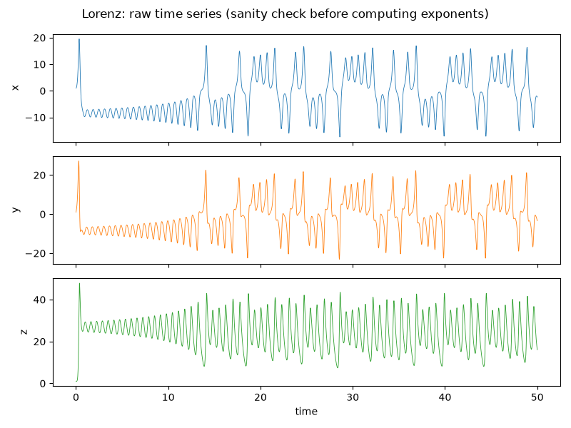
x keeps switching sign as the trajectory hops between the two lobes, and z stays positive – this is the Lorenz attractor behaving as expected. Now compute the exponents from the same problem.

result = lyapunov_spectrum(
    problem, n_steps=50_000, renorm_every=10, t_transient=100.0,
)
print("Lorenz")
print(f"  lambda = {np.array(result.exponents)}")

Lorenz
  lambda = [ 9.01718228e-01  1.66890342e-03 -1.45699518e+01]

Coupled network: same idea, on a step function built with network_problem instead of ode_problem. All-negative Jacobian eigenvalues predict every node decaying toward 0.

weights = np.array([
    [0., 1., 0., 1.],
    [1., 0., 1., 0.],
    [0., 1., 0., 1.],
    [1., 0., 1., 0.],
])
gamma, G = -2.0, 0.5
model = ModelSpec(
    name="linear_node",
    state_variables=(StateVar("x", default_init=0.0),),
    parameters=(Parameter("gamma", gamma),),
    cvar=("x",),
    dfun_str={"x": "gamma * x + c"},
)
dfun = build_jax_dfun(model)
params = {"gamma": gamma, "G": G}
dt_net = 1e-3
network = Network(weights=jnp.array(weights), cvar_indices=model.cvar_indices)
problem_net = network_problem(
    dfun, network, linear_coupling(a=1.0, b=0.0),
    params=params, state0=jnp.array([0.3, -0.1, 0.2, -0.4]), dt=dt_net,
)

n_steps_net = 4_000
t_net, traj_net = simulate_trajectory(
    problem_net.step_fn, problem_net.state0, n_steps_net, dt=dt_net,
)
t_net, traj_net = np.array(t_net), np.array(traj_net)

fig, ax = plt.subplots(figsize=(7, 4))
for i in range(4):
    ax.plot(t_net, traj_net[:, i], label=f"node {i}", color=f"C{i}")
ax.axhline(0.0, color="gray", lw=0.5)
ax.set_xlabel("time")
ax.set_ylabel("x")
ax.set_title("4-node linear network: raw time series (decays to 0, as expected)")
ax.legend()
fig.tight_layout()
plt.show()

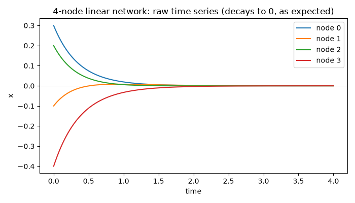
Every node decays toward 0, matching the negative eigenvalues. Same problem, now handed to lyapunov_spectrum.

result_net = lyapunov_spectrum(
    problem_net, n_steps=20_000, renorm_every=10, t_transient=5.0,
)
print("\n4-node linear network")
print(f"  lambda = {np.array(result_net.exponents)}")

4-node linear network
  lambda = [-1.00000336 -1.99999657 -1.99999842 -2.9999943 ]