Linear ODE: exact Lyapunov spectrum

The simplest possible correctness check for the Benettin/QR engine: for a linear system x' = A x, the Lyapunov spectrum is exactly the real parts of the eigenvalues of A – no chaos, no literature value to trust, just linear algebra. See Tier 0.1 of the validation guide.

The system. A here is diagonal with entries -1, -2, -5, so the trajectory decays to the origin along the coordinate axes, and the eigenvalues (already real, since A is diagonal) are exactly -1, -2, -5. Every solution contracts, so all three exponents are negative – there is no chaos to detect, which is the point: this case isolates the numerics of the Lyapunov engine from any question about the dynamics themselves.

The method (Benettin/QR). Alongside the state x(t), lyapax evolves a set of d tangent vectors under the linearized dynamics dY/dt = A Y (for this linear system the “linearization” is just A itself). Left alone, all tangent vectors collapse onto the single fastest-growing (here, slowest-decaying) direction and numerically underflow. To prevent that, every renorm_every steps the tangent matrix Y is QR-decomposed, Y = Q R; Q (an orthonormal basis) replaces Y for the next stretch, and the log of the diagonal of R gives that stretch’s contribution to each exponent. 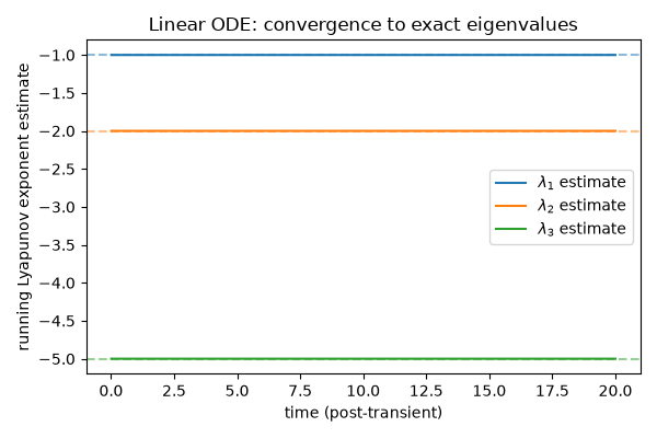Averaging those contributions over time and dividing by elapsed time gives the running estimate plotted below, which converges to Re(eigvals(A)) as the average washes out the initial transient.

import os
import time

os.environ["JAX_PLATFORMS"] = "cpu"

import jax
import jax.numpy as jnp
import matplotlib.pyplot as plt
import numpy as np

jax.config.update("jax_enable_x64", True)

from lyapax import systems
from lyapax.core import lyapunov_spectrum, ode_problem

Distinct real eigenvalues, no coupling, no chaos. ode_problem turns the continuous-time rhs into a fixed-dt update (integrator= "rk4" by default) and bundles state0/dt alongside it, so lyapunov_spectrum – the Benettin/QR engine described above – only needs n_steps and the run controls, not a second copy of dt.

A = jnp.diag(jnp.array([-1.0, -2.0, -5.0]))
rhs = systems.linear_system(A)
dt = 1e-3
problem = ode_problem(rhs, state0=jnp.array([0.3, -0.2, 0.5]), dt=dt)

t0 = time.perf_counter()
result = lyapunov_spectrum(
    problem, n_steps=20_000, renorm_every=10, t_transient=5.0,
)
elapsed = time.perf_counter() - t0

expected = np.array([-1.0, -2.0, -5.0])
estimate = np.array(result.exponents)
print(f"exact eigenvalues:      {expected}")
print(f"lyapax estimate:        {estimate}")
print(f"max abs error:          {np.max(np.abs(estimate - expected)):.2e}")
print(f"wall time (incl. JIT):  {elapsed:.2f}s")

exact eigenvalues:      [-1. -2. -5.]
lyapax estimate:        [-1.00000095 -1.99999905 -5.        ]
max abs error:          9.45e-07
wall time (incl. JIT):  0.67s

Convergence of the running estimate toward the exact eigenvalues. The transient (first 5 time units, not shown) is where the randomly initialized tangent vectors align to the eigendirections – see the note on this in src/lyapax/core.py.

fig, ax = plt.subplots(figsize=(6, 4))
history = np.array(result.history)
times = np.array(result.times)
for i, lam in enumerate(expected):
    ax.plot(times, history[:, i], label=rf"$\lambda_{i + 1}$ estimate", color=f"C{i}")
    ax.axhline(lam, color=f"C{i}", linestyle="--", alpha=0.5)
ax.set_xlabel("time (post-transient)")
ax.set_ylabel("running Lyapunov exponent estimate")
ax.set_title("Linear ODE: convergence to exact eigenvalues")
ax.legend()
fig.tight_layout()
plt.show()