Chaotic flows: Lorenz and Rossler

Full-spectrum Lyapunov exponents for the two classic chaotic-ODE benchmarks, cross-checked against a structural invariant (constant or directly-computable phase-space divergence) as well as published values. See the validation guide, Tier 1 and Tier 2.

The systems. Both are genuinely chaotic, so unlike 01_linear_ode.py and 02_chaotic_maps.py there is no closed-form value for the individual exponents to check against – only a structural invariant plus a published reference value for lambda1. For the Lorenz system, trace(J) = -(sigma + 1 + beta) is constant (state-independent), so the sum of all three exponents is known exactly without running any simulation, no matter how well the attractor itself is resolved – it’s a check on the engine’s overall bookkeeping, not on this particular trajectory. For the Rossler system, trace(J) = a + x - c depends on the state x, so the same check instead needs the trajectory’s time-averaged <x>, computed here from a second, independent run (simulate_trajectory) – a weaker but still exact identity, sum(lambda) = a - c + <x>.

The method. Same Benettin/QR engine as 01_linear_ode.py, just with a nonlinear rhs (linearized freshly at each step via jax.jacfwd, as in 02_chaotic_maps.py) and a much longer transient/run to let the trajectory settle onto the attractor and the running exponent estimates average out their fluctuations – chaotic flows converge far more slowly and noisily than the linear or map examples.

import os
import time

os.environ["JAX_PLATFORMS"] = "cpu"

import jax
import jax.numpy as jnp
import matplotlib.pyplot as plt
import numpy as np

jax.config.update("jax_enable_x64", True)

from lyapax import systems
from lyapax.core import lyapunov_spectrum, ode_problem
from lyapax.utils import simulate_trajectory

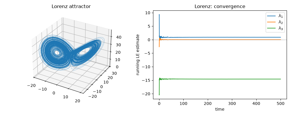
Lorenz: trace(J) = -(sigma + 1 + beta) is constant, so sum(LE) is known exactly regardless of how well the attractor itself is resolved.

sigma, rho, beta = 10.0, 28.0, 8.0 / 3.0
rhs = systems.lorenz(sigma, rho, beta)
dt = 1e-2
problem_lorenz = ode_problem(rhs, state0=jnp.array([1.0, 1.0, 1.0]), dt=dt)

t0 = time.perf_counter()
result_lorenz = lyapunov_spectrum(
    problem_lorenz, n_steps=50_000, renorm_every=10, t_transient=100.0,
)
elapsed_lorenz = time.perf_counter() - t0

expected_sum = -(sigma + 1.0 + beta)
print("Lorenz")
print(f"  lambda        = {np.array(result_lorenz.exponents)}")
print(f"  sum(lambda)   = {float(jnp.sum(result_lorenz.exponents)):.4f}"
      f"   exact -(sigma+1+beta) = {expected_sum:.4f}")
print(f"  lambda1       = {float(result_lorenz.exponents[0]):.4f}   published ~0.9056")
print(f"  wall time     = {elapsed_lorenz:.2f}s (incl. one-time JIT trace/compile)")

Lorenz
  lambda        = [ 9.01718228e-01  1.66890342e-03 -1.45699518e+01]
  sum(lambda)   = -13.6666   exact -(sigma+1+beta) = -13.6667
  lambda1       = 0.9017   published ~0.9056
  wall time     = 0.43s (incl. one-time JIT trace/compile)

traj = np.array(simulate_trajectory(problem_lorenz.step_fn, problem_lorenz.state0, 20_000))

fig = plt.figure(figsize=(10, 4))
ax1 = fig.add_subplot(1, 2, 1, projection="3d")
ax1.plot(traj[:, 0], traj[:, 1], traj[:, 2], lw=0.3)
ax1.set_title("Lorenz attractor")

ax2 = fig.add_subplot(1, 2, 2)
h = np.array(result_lorenz.history)
t = np.array(result_lorenz.times)
for i in range(3):
    ax2.plot(t, h[:, i], label=rf"$\lambda_{i + 1}$")
ax2.axhline(0.0, color="gray", lw=0.5)
ax2.set_xlabel("time")
ax2.set_ylabel("running LE estimate")
ax2.set_title("Lorenz: convergence")
ax2.legend()
fig.tight_layout()
plt.show()

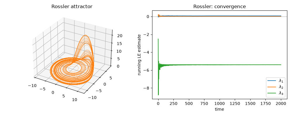
Rossler: trace(J) = a + x - c is not constant, so the invariant check needs the trajectory’s time-average of x from the same run.

a, b, c = 0.2, 0.2, 5.7
rhs = systems.rossler(a, b, c)
problem_rossler = ode_problem(rhs, state0=jnp.array([1.0, 1.0, 1.0]), dt=dt)

result_rossler = lyapunov_spectrum(
    problem_rossler, n_steps=200_000, renorm_every=10, t_transient=200.0,
)

traj_r = np.array(simulate_trajectory(problem_rossler.step_fn, problem_rossler.state0, 50_000))
mean_x = traj_r[:, 0].mean()
expected_sum_rossler = a - c + mean_x

print("\nRossler")
print(f"  lambda            = {np.array(result_rossler.exponents)}")
print(f"  sum(lambda)       = {float(jnp.sum(result_rossler.exponents)):.4f}")
print(f"  a - c + <x>       = {expected_sum_rossler:.4f}   (<x> from a separate trajectory)")
print(f"  lambda1           = {float(result_rossler.exponents[0]):.4f}   published ~0.07")

Rossler
  lambda            = [ 7.07982131e-02 -1.24925864e-04 -5.39916724e+00]
  sum(lambda)       = -5.3285
  a - c + <x>       = -5.3214   (<x> from a separate trajectory)
  lambda1           = 0.0708   published ~0.07

fig = plt.figure(figsize=(10, 4))
ax1 = fig.add_subplot(1, 2, 1, projection="3d")
ax1.plot(traj_r[:, 0], traj_r[:, 1], traj_r[:, 2], lw=0.3, color="C1")
ax1.set_title("Rossler attractor")

ax2 = fig.add_subplot(1, 2, 2)
h = np.array(result_rossler.history)
t = np.array(result_rossler.times)
for i in range(3):
    ax2.plot(t, h[:, i], label=rf"$\lambda_{i + 1}$")
ax2.axhline(0.0, color="gray", lw=0.5)
ax2.set_xlabel("time")
ax2.set_ylabel("running LE estimate")
ax2.set_title("Rossler: convergence")
ax2.legend()
fig.tight_layout()
plt.show()