Differentiating a Lyapunov exponent w.r.t. a system parameter

lyapunov_spectrum is built entirely from jax.lax.scan and jnp.linalg.qr, both of which support ordinary JAX autodiff – so a Lyapunov exponent can be differentiated w.r.t. a system parameter with jax.grad or jax.jacfwd, no different from any other JAX function. The practical payoff: instead of sweeping a parameter and hunting for where an exponent crosses a target value, gradient descent finds it directly – and scales to many parameters at once, where a sweep does not.

The catch. A parameter that the right-hand side closes over also appears inside every step of the trajectory itself, so differentiating the exponent differentiates through the whole unrolled trajectory, not just the tangent-space bookkeeping. For a non-chaotic system that’s harmless. For a genuinely chaotic one, the trajectory is exponentially sensitive to perturbation by construction – and so, therefore, is this gradient. It does not raise an error; it just becomes a large, numerically meaningless number, silently, well before it overflows. This demo shows both sides: gradient-based tuning working cleanly on a non-chaotic system, then the same mechanism breaking down on a chaotic one, measured rather than asserted.

import os

os.environ["JAX_PLATFORMS"] = "cpu"

import jax
import jax.numpy as jnp
import matplotlib.pyplot as plt
import numpy as np

jax.config.update("jax_enable_x64", True)

from lyapax import lyapunov_spectrum, ode_problem, systems

Gradient-based tuning on a non-chaotic system

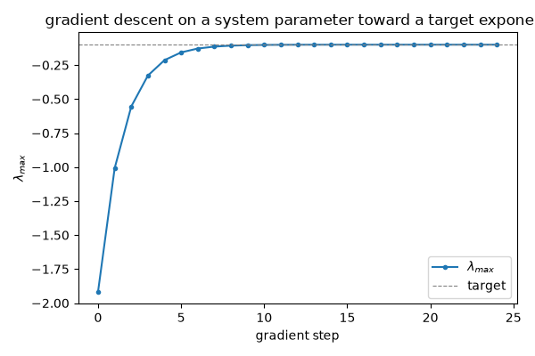
A 2D linear system’s top exponent is exactly its least-negative eigenvalue, gamma. Instead of sweeping gamma to find where lambda_max hits a target value, gradient descent gets there directly.

def lambda_max(gamma):
    def rhs(y):
        return jnp.array([[gamma, 0.5], [-0.5, gamma - 1.0]]) @ y
    problem = ode_problem(rhs, state0=jnp.array([1.0, 0.3]), dt=1e-2, integrator="rk4")
    result = lyapunov_spectrum(problem, n_steps=2_000, renorm_every=1, k=1, t_transient=5.0)
    return result.exponents[0]


target = -0.1
gamma = -1.5
lr = 0.5
history = []
for step in range(25):
    value, grad = jax.value_and_grad(lambda_max)(gamma)
    history.append((step, gamma, float(value)))
    gamma = gamma - lr * (float(value) - target)

print(f"target lambda_max={target}, reached={history[-1][2]:.5f} "
      f"after {len(history)} gradient steps (gamma={history[-1][1]:.4f})")

target lambda_max=-0.1, reached=-0.10000 after 25 gradient steps (gamma=0.3157)

fig, ax = plt.subplots(figsize=(6, 4))
steps, gammas, values = zip(*history)
ax.plot(steps, values, marker="o", ms=3, label=r"$\lambda_{max}$")
ax.axhline(target, color="gray", linestyle="--", linewidth=0.8, label="target")
ax.set_xlabel("gradient step")
ax.set_ylabel(r"$\lambda_{max}$")
ax.set_title("gradient descent on a system parameter toward a target exponent")
ax.legend()
fig.tight_layout()
plt.show()

Reverse-mode (jax.grad) and forward-mode (jax.jacfwd) agree with each other and with a finite-difference reference on this non-chaotic system – there is nothing special about which AD mode is used here.

gamma0 = -0.7
grad_rev = jax.grad(lambda_max)(gamma0)
grad_fwd = jax.jacfwd(lambda_max)(gamma0)
eps = 1e-5
finite_diff = (lambda_max(gamma0 + eps) - lambda_max(gamma0 - eps)) / (2 * eps)
print(f"\ngrad={float(grad_rev):.6f}  jacfwd={float(grad_fwd):.6f}  "
      f"finite_diff={float(finite_diff):.6f}")

grad=1.000000  jacfwd=1.000000  finite_diff=1.000000

The chaotic case: the same gradient becomes meaningless

Now differentiate Lorenz’s leading exponent w.r.t. sigma. The gradient’s magnitude is measured at increasing trajectory lengths – it should stay near some modest, stable sensitivity if it were trustworthy. Instead it grows by many orders of magnitude as the horizon lengthens, tracking the chaotic trajectory’s own exponential divergence rather than any real parameter sensitivity of the long-run exponent.

def lorenz_lambda_max(sigma, n_steps):
    rhs = systems.lorenz(sigma=sigma, rho=28.0, beta=8.0 / 3.0)
    problem = ode_problem(rhs, state0=jnp.array([1.0, 1.0, 1.0]), dt=1e-2, integrator="rk4")
    result = lyapunov_spectrum(problem, n_steps=n_steps, renorm_every=5, k=1, t_transient=20.0)
    return result.exponents[0]


sigma0 = 10.0
horizons = [100, 300, 1_000, 3_000, 10_000]
grad_magnitudes = []
for n_steps in horizons:
    g = jax.grad(lambda s: lorenz_lambda_max(s, n_steps))(sigma0)
    grad_magnitudes.append(abs(float(g)))
    print(f"n_steps={n_steps:6d}  |d(lambda_max)/d(sigma)| = {abs(float(g)):.3e}")

n_steps=   100  |d(lambda_max)/d(sigma)| = 3.332e+03
n_steps=   300  |d(lambda_max)/d(sigma)| = 6.158e+03
n_steps=  1000  |d(lambda_max)/d(sigma)| = 2.720e+06
n_steps=  3000  |d(lambda_max)/d(sigma)| = 4.321e+12
n_steps= 10000  |d(lambda_max)/d(sigma)| = 9.740e+40

fig, ax = plt.subplots(figsize=(6, 4))
ax.semilogy(horizons, grad_magnitudes, marker="o")
ax.set_xlabel("n_steps (trajectory horizon)")
ax.set_ylabel(r"$|d\lambda_{max}/d\sigma|$ (log scale)")
ax.set_title("chaotic-trajectory gradient blows up with horizon length")
fig.tight_layout()
plt.show()

print(
    "\nTakeaway: jax.grad/jax.jacfwd through lyapunov_spectrum are reliable "
    "for non-chaotic or short-horizon systems (as in the gradient-descent "
    "example above), but a gradient computed through a long chaotic "
    "trajectory should not be trusted without an independent check, e.g. "
    "against a finite-difference reference."
)

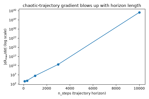
Takeaway: jax.grad/jax.jacfwd through lyapunov_spectrum are reliable for non-chaotic or short-horizon systems (as in the gradient-descent example above), but a gradient computed through a long chaotic trajectory should not be trusted without an independent check, e.g. against a finite-difference reference.