Coupled linear network: exact eigenvalues

Isolates “did we wire the coupling term into the Jacobian correctly” from “is chaos numerically well-resolved”: for a linear coupled network, the full Lyapunov spectrum is exactly the eigenvalues of the constant network Jacobian gamma*I + G*W. See Tier 3 of the validation guide.

The system. Each of the 4 nodes has identical scalar linear dynamics x_i' = gamma * x_i + c_i, where c_i is the coupling input from its neighbors; with linear_coupling(a=1, b=0) that input is c_i = G * sum_j w[i, j] x_j, i.e. a matrix-vector product against the adjacency matrix W. Stacking all nodes, the whole network is therefore the single linear ODE x' = (gamma*I + G*W) x – the same kind of exact eigenvalue check as 01_linear_ode.py, except now A is assembled from a graph and a coupling rule instead of being handed to the engine directly, so this validates that assembly rather than the core QR bookkeeping. 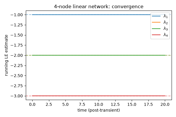W here is a 4-node cycle graph (a-b-c-d-a), which is symmetric (so real eigenvalues) with known spectrum {2, 0, 0, -2}; shifting and scaling by gamma=-2, G=0.5 gives A’s eigenvalues {-1, -2, -2, -3}.

The machinery. ModelSpec/build_jax_dfun (vendored from vbi, see src/lyapax/simulator/NOTICE.md) compile a symbolic per-node right-hand side – here the string "gamma * x + c" – into a JAX function, rather than hand-writing the node dynamics as in the earlier examples; c is always the coupling input. A lyapax.Network names the topology (weights, cvar_indices), and network_problem wires that dfun together with a coupling (see lyapax.coupling – here linear_coupling, matching the identity coupling assumed above) and a Heun integrator into the flat state -> new_state function lyapunov_spectrum expects, reshaping between the network’s natural (n_state_vars, n_nodes) layout and the flat vector the QR engine operates on – while also bundling state0/dt alongside it, the same problem-object recipe ode_problem gives the plain-ODE case in 01_linear_ode.py.

import os

os.environ["JAX_PLATFORMS"] = "cpu"
import jax
import jax.numpy as jnp
import matplotlib.pyplot as plt
import numpy as np

jax.config.update("jax_enable_x64", True)

from lyapax.core import lyapunov_spectrum
from lyapax.coupling import linear_coupling
from lyapax.network import Network, network_problem
from lyapax.simulator import ModelSpec, Parameter, StateVar, build_jax_dfun

4-cycle graph adjacency (symmetric -> real eigenvalues): {2, 0, 0, -2}.

weights = np.array([
    [0., 1., 0., 1.],
    [1., 0., 1., 0.],
    [0., 1., 0., 1.],
    [1., 0., 1., 0.],
])
gamma, G = -2.0, 0.5
A = gamma * np.eye(4) + G * weights
expected = np.sort(np.linalg.eigvalsh(A))[::-1]

model = ModelSpec(
    name="linear_node",
    state_variables=(StateVar("x", default_init=0.0),),
    parameters=(Parameter("gamma", gamma),),
    cvar=("x",),
    dfun_str={"x": "gamma * x + c"},
)
dfun = build_jax_dfun(model)
params = {"gamma": gamma, "G": G}
dt = 1e-3
network = Network(weights=jnp.array(weights), cvar_indices=model.cvar_indices)
problem = network_problem(
    dfun, network, linear_coupling(a=1.0, b=0.0),
    params=params, state0=jnp.array([0.3, -0.1, 0.2, -0.4]), dt=dt,
)

result = lyapunov_spectrum(
    problem, n_steps=20_000, renorm_every=10, t_transient=5.0,
)

estimate = np.array(result.exponents)
print(f"exact eigenvalues:  {expected}")
print(f"lyapax estimate:    {estimate}")
print(f"max abs error:      {np.max(np.abs(estimate - expected)):.2e}")

exact eigenvalues:  [-1. -2. -2. -3.]
lyapax estimate:    [-1.00000336 -1.99999657 -1.99999842 -2.9999943 ]
max abs error:      5.70e-06

fig, ax = plt.subplots(figsize=(6, 4))
h = np.array(result.history)
t = np.array(result.times)
for i, lam in enumerate(expected):
    ax.plot(t, h[:, i], label=rf"$\lambda_{i + 1}$", color=f"C{i}")
    ax.axhline(lam, color=f"C{i}", linestyle="--", alpha=0.5)
ax.set_xlabel("time (post-transient)")
ax.set_ylabel("running LE estimate")
ax.set_title("4-node linear network: convergence")
ax.legend()
fig.tight_layout()
plt.show()