Kuramoto network with delayed coupling: what transmission delay does

Extends 05_kuramoto_sync.py’s zero-delay synchronization sweep to a delayed Kuramoto network – the same 6-oscillator, heterogeneous- frequency, all-to-all system, but now each oscillator feels its neighbors’ phases as they were tau time units ago rather than instantaneously, via dtheta_i/dt = omega_i + (G/N) sum_j sin(theta_j(t-tau) - theta_i(t)). Runs the same G sweep two ways – zero delay (exactly 05_kuramoto_sync.py) and tau=0.3 (the delayed/DDE engine) – and overlays lambda_2 from both, since lambda_2 is what tracks synchronization (see 05_kuramoto_sync.py’s docstring for why: lambda_1 is pinned to 0 by the model’s exact rotational symmetry and never signals anything).

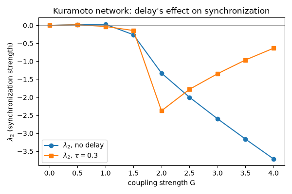
What to expect, and why. At G=0 both delayed and undelayed networks are decoupled oscillators (dtheta/dt=omega, state-independent regardless of delay), so every exponent is exactly 0 either way – this is checked numerically below, not just asserted. Away from G=0, a finite transmission delay is well known (e.g. in Kuramoto-with-delay studies) to act against synchronization: information about a neighbor’s phase arrives stale, weakening the effective restoring force, so reaching the same degree of lock (same lambda_2) generally needs more coupling with delay than without. Whether that shift is large or small here is an empirical question this script answers for these specific parameters, not a foregone conclusion – read the printed/plotted lambda_2 curves rather than assuming the story below.

The machinery. Both runs share the same ModelSpec/dfun ("omega + c") and kuramoto_coupling callable as 05_kuramoto_sync.py, wired through one shared lyapax.Network topology object – lyapax.coupling builders are plain callables with no delay opinion baked in, so the same coupling function works whether the state it receives is instantaneous or delayed. The delay-0 run goes through lyapax.network_problem + lyapax.lyapunov_spectrum, the same front door 05_kuramoto_sync.py itself now uses, so the two produce exactly the same numbers; the delayed run goes through lyapax.network_dde_problem(..., tau=tau) (the uniform-delay branch – a single global tau shared by every edge, not the per-edge delay_steps matrix from 08_delayed_coupling.py) + lyapax.lyapunov_spectrum_dde. Both problem constructors are thin wrappers that build the ring buffer and resolve tau to whole dt steps for you – see 12_public_api_overview.py for the general problem-object recipe.

Note: like 05_kuramoto_sync.py, this sweeps G with a Python loop, one lyapunov_spectrum[_dde] call per point (see 11_vmap_parameter_sweep.py for the batched-vmap alternative on the zero-delay engine). The delayed engine’s tangent propagation costs O(k) forward passes per raw step (via jax.jvp/jax.vmap, not a dense Jacobian – see lyapax/dde.py’s module docstring), which is why this is tractable at all despite the ring buffer adding horizon * n_nodes extra tangent-carried dimensions per node.

import os

os.environ["JAX_PLATFORMS"] = "cpu"
import time

import jax
import jax.numpy as jnp
import matplotlib.pyplot as plt
import numpy as np

jax.config.update("jax_enable_x64", True)

import lyapax
from lyapax.coupling import kuramoto_coupling
from lyapax.simulator import ModelSpec, Parameter, StateVar, build_jax_dfun

n_nodes = 6
omega = jnp.linspace(-1.0, 1.0, n_nodes)
weights = jnp.ones((n_nodes, n_nodes)) - jnp.eye(n_nodes)

model = ModelSpec(
    name="kuramoto",
    state_variables=(StateVar("theta", default_init=0.0),),
    parameters=(Parameter("omega", 0.0),),
    cvar=("theta",),
    dfun_str={"theta": "omega + c"},
)
dfun = build_jax_dfun(model)
network = lyapax.Network(weights=weights, cvar_indices=model.cvar_indices)

dt = 1e-2
tau = 0.3
state0 = jnp.linspace(0.0, 2 * jnp.pi, n_nodes, endpoint=False)

G_values = np.linspace(0.0, 4.0, 9)
lambda2_nodelay, lambda2_delayed = [], []

t0 = time.perf_counter()
for G in G_values:
    params = {"omega": omega, "G": float(G)}

    # -- zero delay: exactly 05_kuramoto_sync.py's engine, via the network_problem front door --
    problem_nodelay = lyapax.network_problem(
        dfun, network, kuramoto_coupling(alpha=0.0),
        params=params, state0=state0, dt=dt,
    )
    result_nodelay = lyapax.lyapunov_spectrum(
        problem_nodelay, n_steps=4_000, renorm_every=10, k=2, t_transient=20.0,
    )
    lambda2_nodelay.append(float(result_nodelay.exponents[1]))

    # -- uniform delay tau=0.3: the DDE engine, via network_dde_problem --
    problem_delayed = lyapax.network_dde_problem(
        dfun, network, kuramoto_coupling(alpha=0.0),
        params=params, state0=state0.reshape(1, n_nodes), dt=dt, tau=tau,
        integrator="heun",
    )
    result_delayed = lyapax.lyapunov_spectrum_dde(
        problem_delayed, n_steps=4_000, k=2, renorm_every=10, t_transient=20.0,
    )
    lambda2_delayed.append(float(result_delayed.exponents[1]))
elapsed = time.perf_counter() - t0
print(f"swept {len(G_values)} values of G (2 engines each) in {elapsed:.1f}s "
      f"({elapsed / (2 * len(G_values)):.2f}s/run)")
print(f"G=0 sanity check (should be exactly 0 either way): "
      f"no-delay lambda2={lambda2_nodelay[0]:.2e}, "
      f"delayed lambda2={lambda2_delayed[0]:.2e}")
for G, l2_nd, l2_d in zip(G_values, lambda2_nodelay, lambda2_delayed):
    print(f"  G={G:.2f}  lambda2 (no delay)={l2_nd:+.4f}  lambda2 (tau={tau})={l2_d:+.4f}")

swept 9 values of G (2 engines each) in 11.6s (0.65s/run)
G=0 sanity check (should be exactly 0 either way): no-delay lambda2=0.00e+00, delayed lambda2=0.00e+00
  G=0.00  lambda2 (no delay)=+0.0000  lambda2 (tau=0.3)=+0.0000
  G=0.50  lambda2 (no delay)=+0.0201  lambda2 (tau=0.3)=+0.0150
  G=1.00  lambda2 (no delay)=+0.0278  lambda2 (tau=0.3)=-0.0313
  G=1.50  lambda2 (no delay)=-0.2609  lambda2 (tau=0.3)=-0.1435
  G=2.00  lambda2 (no delay)=-1.3269  lambda2 (tau=0.3)=-2.3753
  G=2.50  lambda2 (no delay)=-1.9984  lambda2 (tau=0.3)=-1.7780
  G=3.00  lambda2 (no delay)=-2.5959  lambda2 (tau=0.3)=-1.3454
  G=3.50  lambda2 (no delay)=-3.1621  lambda2 (tau=0.3)=-0.9620
  G=4.00  lambda2 (no delay)=-3.7121  lambda2 (tau=0.3)=-0.6362

fig, ax = plt.subplots(figsize=(6, 4))
ax.plot(G_values, lambda2_nodelay, "o-", label=r"$\lambda_2$, no delay")
ax.plot(G_values, lambda2_delayed, "s-", label=rf"$\lambda_2$, $\tau={tau}$")
ax.axhline(0.0, color="gray", lw=0.5)
ax.set_xlabel("coupling strength G")
ax.set_ylabel(r"$\lambda_2$ (synchronization strength)")
ax.set_title("Kuramoto network: delay's effect on synchronization")
ax.legend()
fig.tight_layout()
plt.show()