Kuramoto network: synchronization transition

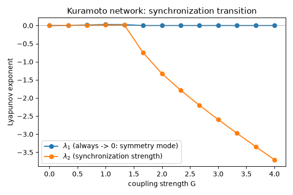
Sweeps the global coupling strength G and tracks the top two Lyapunov exponents of a small heterogeneous-frequency Kuramoto network. At G=0 both are exactly 0 (decoupled oscillators: dtheta/dt = omega is state-independent, so the step map’s Jacobian is exactly the identity – see tests/test_network.py::test_kuramoto_zero_coupling_gives_exactly_zero_spectrum).

The Kuramoto model has an exact continuous symmetry (theta_i -> theta_i + c for all i leaves the dynamics unchanged), which guarantees one Lyapunov exponent stays exactly 0 once phase-locked – it never goes negative. What actually signals synchronization is lambda_2: below threshold both leading exponents are small and positive (weakly unstable/incoherent regime); once the network locks, lambda_1 snaps to machine-precision 0 (the marginal rotation mode) and lambda_2 turns negative, growing more negative as coupling strengthens the lock. This is exactly what the run below shows – not a hypothesis, it’s what lyapax actually produces for this network.

Note: this sweep calls lyapunov_spectrum once per G value in a plain Python loop; see examples/11_vmap_parameter_sweep.py for the same sweep done as a single batched jax.vmap call instead, and examples/07_speed_and_accuracy.py for what the per-call cost is.

The system. 6 oscillators, all-to-all coupled (weights is the complete graph: 1 everywhere off the diagonal, 0 on it), with heterogeneous natural frequencies omega evenly spaced over [-1, 1] so the population would never sync on its own – staggered initial phases start it far from the locked state. The classic Kuramoto ODE dtheta_i/dt = omega_i + (G/N) sum_j sin(theta_j - theta_i) is built here from the same machinery as 04_linear_network.py: ModelSpec/build_jax_dfun compile the bare node dynamics "omega + c" (c is the coupling input) into a JAX function, and kuramoto_coupling supplies the sine-coupling term as c; network_problem wires the two together (plus a lyapax.Network topology and state0/dt) into the flat step function the Lyapunov engine steps. Only k=2 exponents are tracked per run (not the full spectrum of 6) since only the top two are needed to read off the transition – see the k parameter in lyapunov_spectrum’s docstring for the leading-exponents-only cost tradeoff.

import os

os.environ["JAX_PLATFORMS"] = "cpu"
import time

import jax
import jax.numpy as jnp
import matplotlib.pyplot as plt
import numpy as np

jax.config.update("jax_enable_x64", True)

from lyapax.core import lyapunov_spectrum
from lyapax.coupling import kuramoto_coupling
from lyapax.network import Network, network_problem
from lyapax.simulator import ModelSpec, Parameter, StateVar, build_jax_dfun

n_nodes = 6
omega = jnp.linspace(-1.0, 1.0, n_nodes)
weights = jnp.ones((n_nodes, n_nodes)) - jnp.eye(n_nodes)

model = ModelSpec(
    name="kuramoto",
    state_variables=(StateVar("theta", default_init=0.0),),
    parameters=(Parameter("omega", 0.0),),
    cvar=("theta",),
    dfun_str={"theta": "omega + c"},
)
dfun = build_jax_dfun(model)
network = Network(weights=weights, cvar_indices=model.cvar_indices)

dt = 1e-2
state0 = jnp.linspace(0.0, 2 * jnp.pi, n_nodes, endpoint=False)

G_values = np.linspace(0.0, 4.0, 13)
lambda1, lambda2 = [], []

t0 = time.perf_counter()
for G in G_values:
    params = {"omega": omega, "G": float(G)}
    problem = network_problem(
        dfun, network, kuramoto_coupling(alpha=0.0),
        params=params, state0=state0, dt=dt,
    )
    result = lyapunov_spectrum(
        problem, n_steps=5_000, renorm_every=10, k=2, t_transient=50.0,
    )
    lambda1.append(float(result.exponents[0]))
    lambda2.append(float(result.exponents[1]))
elapsed = time.perf_counter() - t0
print(f"swept {len(G_values)} values of G in {elapsed:.1f}s "
      f"({elapsed / len(G_values):.2f}s/run)")
for G, l1, l2 in zip(G_values, lambda1, lambda2):
    print(f"  G={G:.2f}  lambda1={l1:+.4f}  lambda2={l2:+.4f}")

swept 13 values of G in 5.8s (0.45s/run)
  G=0.00  lambda1=+0.0000  lambda2=+0.0000
  G=0.33  lambda1=+0.0040  lambda2=+0.0034
  G=0.67  lambda1=+0.0126  lambda2=+0.0070
  G=1.00  lambda1=+0.0289  lambda2=+0.0121
  G=1.33  lambda1=+0.0243  lambda2=+0.0116
  G=1.67  lambda1=+0.0000  lambda2=-0.7518
  G=2.00  lambda1=+0.0000  lambda2=-1.3269
  G=2.33  lambda1=+0.0000  lambda2=-1.7867
  G=2.67  lambda1=+0.0000  lambda2=-2.2025
  G=3.00  lambda1=+0.0000  lambda2=-2.5951
  G=3.33  lambda1=+0.0000  lambda2=-2.9734
  G=3.67  lambda1=+0.0000  lambda2=-3.3423
  G=4.00  lambda1=+0.0000  lambda2=-3.7044

fig, ax = plt.subplots(figsize=(6, 4))
ax.plot(G_values, lambda1, "o-", label=r"$\lambda_1$ (always -> 0: symmetry mode)")
ax.plot(G_values, lambda2, "o-", label=r"$\lambda_2$ (synchronization strength)")
ax.axhline(0.0, color="gray", lw=0.5)
ax.set_xlabel("coupling strength G")
ax.set_ylabel("Lyapunov exponent")
ax.set_title("Kuramoto network: synchronization transition")
ax.legend()
fig.tight_layout()
plt.show()