
Lyapunov exponents#
This page explains what Lyapunov exponents are, how a computed spectrum can be sanity-checked, and the Benettin/QR algorithm that lyapax implements. For a book-length treatment, see Pikovsky & Politi [9]; for a compact survey of the theory and the numerical methods, see Skokos [8].
What a Lyapunov exponent measures#
Consider a dynamical system
or a discrete map \(x_{n+1} = F(x_n)\). The Lyapunov exponents \(\lambda_1 \ge \lambda_2 \ge \dots \ge \lambda_d\) measure the average exponential rate at which infinitesimally close trajectories separate (positive exponent) or converge (negative exponent) along each of \(d\) independent directions in state space.
Formally, linearize around a reference trajectory \(x(t)\): an infinitesimal perturbation \(\delta x(t)\) evolves under the variational (tangent) equation
and the \(i\)-th Lyapunov exponent is the long-time average growth rate of the \(i\)-th ordered singular direction of the tangent flow,
where \(\sigma_i(T)\) are the singular values of the linearized flow map over \([0, T]\). That this limit exists for almost every initial condition (with respect to an ergodic invariant measure) is the content of Oseledets’ multiplicative ergodic theorem [1]; the connection between Lyapunov exponents, ergodic theory, and strange attractors is reviewed by Eckmann & Ruelle [2].
In practice nobody evaluates that limit or that SVD directly: a single generic perturbation collapses onto the fastest-growing direction almost immediately, and everything overflows or underflows in finite precision. Every practical algorithm therefore periodically re-orthonormalizes a whole basis of perturbation vectors instead of tracking one - that is the Benettin/QR method described below.
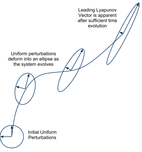
Growth of perturbations along a trajectory, the local object averaged by Lyapunov exponents. Image: Mrocklin, Wikimedia Commons, CC BY-SA 3.0.#

Reading a spectrum: structural checks#
A few structural facts make Lyapunov spectra checkable, independent of whether the underlying system is chaotic:
Sign meaning. At least one positive exponent is the standard operational definition of chaos - sensitive dependence on initial conditions [2]. An all-negative spectrum means the trajectory converges to a fixed point or a stable limit cycle. A zero exponent along the flow direction is generic for any bounded continuous-time attractor that is not a fixed point: perturbing along the trajectory itself neither grows nor shrinks [4].
Sum invariant. The exponents satisfy \(\sum_i \lambda_i = \lim_{T\to\infty} \frac{1}{T} \int_0^T \operatorname{tr} J(x(t)) \, dt\), the time-averaged divergence of the flow. For systems where \(\operatorname{tr} J\) is constant - the Lorenz system is the classic case - the sum is known exactly with no simulation at all; for others (e.g. Rössler) it reduces to a time average of one state variable, checkable from an independently computed trajectory. lyapax’s own test suite is anchored to checks of exactly this kind, plus closed-form and published literature values [4], because for a generic chaotic system there is no ground-truth oracle to compare against.
Continuous symmetry → exact zero exponent. If the dynamics are invariant under a continuous transformation - for example Kuramoto phases under a global rotation \(\theta_i \to \theta_i + c\) - the generator of that symmetry is an exactly marginal direction: one exponent is pinned to \(0\), never negative, regardless of parameters. This is a model-specific but very sharp correctness check, used throughout the Kuramoto examples in the gallery.
The Benettin/QR method#
lyapax uses the standard variational (tangent-space) approach with periodic reorthonormalization, introduced by Benettin, Galgani, Giorgilli & Strelcyn [3] and, independently, by Shimada & Nagashima [5]. The reorthonormalization is expressed as a QR decomposition, which computes the full spectrum - not just the leading exponent. Wolf et al. [4] popularized the Gram–Schmidt variant of the same idea; Geist, Parlitz & Lauterborn [6] compare this family of methods systematically, and Sandri [7] gives a readable worked implementation.
The algorithm, as implemented in
lyapax.lyapunov_spectrum:
Propagate the state \(x\) forward one step at a time under the chosen fixed-step map (Euler / Heun / RK4 / RK6, or one iterate of a discrete map).
Alongside it, propagate a \((d, k)\) matrix \(Y\) of tangent vectors under the same step’s linearization. Here \(k \le d\) is how many leading exponents are tracked; \(k = d\) gives the full spectrum.
Every
renorm_everysteps, QR-decompose \(Y = QR\). The orthonormal factor \(Q\) replaces \(Y\) for the next stretch, and \(\log \lvert \operatorname{diag} R \rvert\) for that stretch is accumulated per column.Dividing each column’s running sum by the elapsed time gives its Lyapunov exponent estimate. The estimate converges as the initial-condition-dependent transient washes out (discarded via
t_transient) and the running average smooths over the trajectory’s natural fluctuations.
Two practical caveats follow directly from the construction:
The exponents are those of the numerical time-
dtmap, not of the exact continuous flow. Checking that results are converged indtis the caller’s responsibility.The estimate at finite \(T\) fluctuates around its limit; judge convergence from the running history rather than from a single final number.
Delay systems#
A delay differential equation \(\dot{x}(t) = f(x(t), x(t-\tau))\) is formally an infinite-dimensional dynamical system: its state is a whole history segment, not a point in \(\mathbb{R}^d\). Lyapunov spectra for such systems are nonetheless well defined and computable by discretizing the history, as first demonstrated by Farmer for the Mackey–Glass equation [10]. lyapax follows the same idea: the Benettin/QR machinery above is applied to an augmented carry containing the current state plus a fixed-depth ring buffer of recent history, and the tangent dynamics are differentiated through both jointly - a delayed sensitivity \(\partial f / \partial x(t-\tau)\) is exactly as real as the instantaneous one, and dropping it gives wrong exponents, not just imprecise ones.
References#
V. I. Oseledets, A multiplicative ergodic theorem. Lyapunov characteristic numbers for dynamical systems, Transactions of the Moscow Mathematical Society 19 (1968) 197–231.
J.-P. Eckmann and D. Ruelle, Ergodic theory of chaos and strange attractors, Reviews of Modern Physics 57 (1985) 617–656. doi:10.1103/RevModPhys.57.617
G. Benettin, L. Galgani, A. Giorgilli, and J.-M. Strelcyn, Lyapunov characteristic exponents for smooth dynamical systems and for Hamiltonian systems; a method for computing all of them, Parts 1 and 2, Meccanica 15 (1980) 9–20 and 21–30. doi:10.1007/BF02128236, doi:10.1007/BF02128237
A. Wolf, J. B. Swift, H. L. Swinney, and J. A. Vastano, Determining Lyapunov exponents from a time series, Physica D 16 (1985) 285–317. doi:10.1016/0167-2789(85)90011-9
I. Shimada and T. Nagashima, A numerical approach to ergodic problem of dissipative dynamical systems, Progress of Theoretical Physics 61 (1979) 1605–1616. doi:10.1143/PTP.61.1605
K. Geist, U. Parlitz, and W. Lauterborn, Comparison of different methods for computing Lyapunov exponents, Progress of Theoretical Physics 83 (1990) 875–893. doi:10.1143/PTP.83.875
M. Sandri, Numerical calculation of Lyapunov exponents, The Mathematica Journal 6 (1996) 78–84.
Ch. Skokos, The Lyapunov characteristic exponents and their computation, Lecture Notes in Physics 790 (2010) 63–135. doi:10.1007/978-3-642-04458-8_2 (also arXiv:0811.0882)
A. Pikovsky and A. Politi, Lyapunov Exponents: A Tool to Explore Complex Dynamics, Cambridge University Press, 2016. doi:10.1017/CBO9781139343473
J. D. Farmer, Chaotic attractors of an infinite-dimensional dynamical system, Physica D 4 (1982) 366–393. doi:10.1016/0167-2789(82)90042-2