Chaotic maps: exact analytic Lyapunov exponents

Discrete maps avoid integration-scheme error entirely – useful for isolating bugs in the QR/renormalization bookkeeping itself, independent of any ODE-integrator accuracy question. See the validation guide, Tier 0.2 and Tier 0.3.

The systems. The logistic map x_{n+1} = r x_n (1 - x_n) at r=4 is exactly conjugate to the tent map via x = sin^2(pi y / 2), which gives its Lyapunov exponent in closed form: ln(2). The Henon map (x, y) -> (1 - a x^2 + y, b x) is chaotic for the classic parameters a=1.4, b=0.3 and has no closed-form individual exponents, but its Jacobian [[-2ax, 1], [b, 0]] has constant determinant -b at every point, so the sum of its two exponents is pinned exactly to ln|b| – a structural invariant that holds regardless of how chaotic the individual directions are.

The method. Unlike the ODE example, there is no integrator here: each map is already a one-step update, so lyapunov_spectrum calls jax.jacfwd(step_fn) directly on the map at every step to linearize it, then evolves the tangent (deviation-vector) matrix under that Jacobian and periodically re-orthonormalizes it via QR decomposition (the Benettin/QR method – see 01_linear_ode.py for the full mechanics). Passing dt=1.0 just labels each map iterate as one time unit, so the resulting exponents are directly per-iterate growth rates.

import os

os.environ["JAX_PLATFORMS"] = "cpu"

import jax
import jax.numpy as jnp
import matplotlib.pyplot as plt
import numpy as np

jax.config.update("jax_enable_x64", True)

from lyapax import systems
from lyapax.core import lyapunov_spectrum

Logistic map at r=4: exactly conjugate to the tent map, exact LE = ln(2). renorm_every=1: unlike a fine ODE substep, one map iterate can already stretch a tangent vector by a large factor, so QR after every single step keeps the running product well within float64 range.

step = systems.logistic_map(r=4.0)
result_logistic = lyapunov_spectrum(
    step, state0=jnp.array([0.4]),
    dt=1.0, n_steps=500_000, renorm_every=1, t_transient=1_000.0,
)
print(f"logistic map (r=4):  estimate={float(result_logistic.exponents[0]):.6f}"
      f"  exact=ln(2)={np.log(2):.6f}")

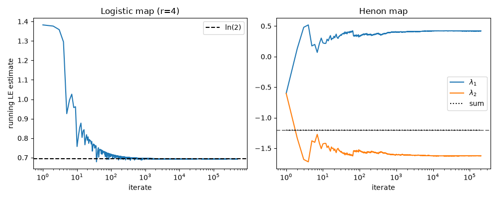
logistic map (r=4):  estimate=0.693152  exact=ln(2)=0.693147

Henon map: the Jacobian determinant is the constant -b, so sum(LE) = ln|b| exactly, independent of the individual exponents’ values. This is the k=None (full-spectrum) default of lyapunov_spectrum, since the sum check needs both exponents, not just the leading one.

a, b = 1.4, 0.3
step = systems.henon_map(a=a, b=b)
result_henon = lyapunov_spectrum(
    step, state0=jnp.array([0.1, 0.1]),
    dt=1.0, n_steps=200_000, renorm_every=1, t_transient=1_000.0,
)
total = float(jnp.sum(result_henon.exponents))
print(f"Henon map:  lambda1={float(result_henon.exponents[0]):.4f}"
      f"  lambda2={float(result_henon.exponents[1]):.4f}")
print(f"Henon map:  sum={total:.6f}  exact=ln(0.3)={np.log(0.3):.6f}")

Henon map:  lambda1=0.4193  lambda2=-1.6233
Henon map:  sum=-1.203973  exact=ln(0.3)=-1.203973

fig, axes = plt.subplots(1, 2, figsize=(10, 4))

h = np.array(result_logistic.history)
t = np.array(result_logistic.times)
axes[0].plot(t, h[:, 0])
axes[0].axhline(np.log(2), color="k", linestyle="--", label="ln(2)")
axes[0].set_xscale("log")
axes[0].set_title("Logistic map (r=4)")
axes[0].set_xlabel("iterate")
axes[0].set_ylabel("running LE estimate")
axes[0].legend()

h = np.array(result_henon.history)
t = np.array(result_henon.times)
axes[1].plot(t, h[:, 0], label=r"$\lambda_1$")
axes[1].plot(t, h[:, 1], label=r"$\lambda_2$")
axes[1].plot(t, h.sum(axis=1), label="sum", color="k", linestyle=":")
axes[1].axhline(np.log(0.3), color="k", linestyle="--", alpha=0.5)
axes[1].set_xscale("log")
axes[1].set_title("Henon map")
axes[1].set_xlabel("iterate")
axes[1].legend()

fig.tight_layout()
plt.show()