DDE history reads: grid-snapped vs Hermite-interpolated

Every delayed-coupling example so far has read history off an exact ring- buffer grid point: the physical delay tau is rounded to the nearest whole number of dt steps before the run even starts (resolve_tau_steps), and every later lookup pulls that exact stored sample. That’s simple and fully differentiable, but it means the delay actually being simulated is tau_eff = tau_steps * dt, not the tau that was asked for – and, because rounding to the nearest integer is not a smooth function of dt, the size of that mismatch does not shrink smoothly as dt gets finer. It can even get worse at a smaller dt if the rounding happens to land less favorably there than at a coarser one.

lyapax.dde_problem(..., interpolate=True) (and its networked counterpart, network_dde_problem) removes the rounding: instead of reading one stored ring-buffer sample, it reconstructs the delayed value via a cubic Hermite interpolant built from the value and derivative stored at the two grid points bracketing the exact delayed time. tau is then used exactly – no snapping, no warning – and refining dt gives a smooth, monotonically shrinking error instead of a jumpy one.

The test system. The scalar linear DDE x'(t) = -a*x(t-tau) has a transcendental characteristic equation whose dominant root is a Lambert-W expression, giving an exact reference Lyapunov exponent to compare against at every dt – the same system used in 01_linear_ode.py’s non-delayed counterpart, but here it lets this demo measure how the error behaves as dt shrinks, not just its size at one dt.

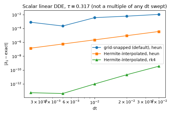
Reading the plot. The grid-snapped curve should look noticeably less smooth than the interpolated ones – not simply “bigger error”, but visibly non-monotonic in places, since its error is dominated by which way tau/dt happens to round at each dt, not by a shrinking numerical truncation error. The interpolated curves should look like clean, (roughly) straight lines on log-log axes instead: slope ~2 for heun, and visibly steeper (~4) for rk4 until it hits the estimation noise floor.

Convergence order. Interpolation buys more than exactness in tau: because the stored (value, derivative) pairs let the delayed value be reconstructed at any time, each integrator stage reads the history at its own intra-step time instead of freezing one read across the whole step. Freezing is an O(dt) error in the delayed argument, and it used to cap every integrator at first order for any delayed system regardless of the method’s nominal order. With per-stage reads, the integrator’s real order is realized: the interpolated curve below should show a slope close to 2 on log-log axes (heun’s nominal order), and switching to integrator="rk4" steepens it to ~4 – the cubic Hermite interpolant’s own accuracy ceiling, so rk6 buys nothing further for a DDE. The grid-snapped default has no sub-step history to read, so it stays O(dt) (on top of its non-monotonic tau-rounding error).

import os
import warnings

os.environ["JAX_PLATFORMS"] = "cpu"

import jax
import jax.numpy as jnp
import matplotlib.pyplot as plt
from scipy.special import lambertw

jax.config.update("jax_enable_x64", True)

from lyapax import systems
from lyapax.dde import dde_problem, lyapunov_spectrum_dde

a = 0.5
tau = 0.317  # deliberately not a clean multiple of any dt swept below
rhs = systems.linear_scalar_dde(a=a)
expected = float((lambertw(-a * tau, k=0) / tau).real)
print(f"exact dominant exponent (Lambert W): {expected:.6f}")

dts = [4e-2, 2e-2, 1e-2, 5e-3, 2.5e-3]
n_steps, renorm_every, t_transient = 40_000, 5, 20.0


def _run(interpolate, integrator="heun"):
    errors, tau_used = [], []
    for dt in dts:
        # The grid-snapped runs warn that tau rounds to tau_eff != tau at
        # every dt here -- that mismatch is exactly what this demo measures
        # (see the tau_eff column in the printed table), so the expected
        # warning is silenced rather than repeated five times.
        with warnings.catch_warnings():
            warnings.filterwarnings("ignore", message="resolve_tau_steps")
            problem = dde_problem(
                rhs, state0=jnp.array([1.0]), tau=tau, dt=dt,
                integrator=integrator, interpolate=interpolate,
            )
        result = lyapunov_spectrum_dde(
            problem, n_steps=n_steps, k=1, renorm_every=renorm_every,
            t_transient=t_transient,
        )
        errors.append(abs(float(result.exponents[0]) - expected))
        tau_used.append(problem.tau_steps * dt)
    return errors, tau_used


errors_snap, tau_eff_snap = _run(interpolate=False)
errors_interp, tau_eff_interp = _run(interpolate=True)
errors_interp_rk4, _ = _run(interpolate=True, integrator="rk4")

print(f"\n{'dt':>8}  {'tau_eff (snap)':>14}  {'err (snap)':>11}  "
      f"{'tau_eff (interp)':>16}  {'err (interp)':>13}")
for dt, te_s, e_s, te_i, e_i in zip(
        dts, tau_eff_snap, errors_snap, tau_eff_interp, errors_interp):
    print(f"{dt:8.4f}  {te_s:14.5f}  {e_s:11.2e}  {te_i:16.5f}  {e_i:13.2e}")

exact dominant exponent (Lambert W): -0.605873

      dt  tau_eff (snap)   err (snap)  tau_eff (interp)   err (interp)
  0.0400         0.32000     1.07e-02           0.31700       3.68e-05
  0.0200         0.32000     6.00e-03           0.31700       9.19e-06
  0.0100         0.32000     3.67e-03           0.31700       2.30e-06
  0.0050         0.31500     2.27e-04           0.31700       5.73e-07
  0.0025         0.31750     7.97e-04           0.31700       1.43e-07

fig, ax = plt.subplots(figsize=(6, 4))
ax.loglog(dts, errors_snap, "o-", label="grid-snapped (default), heun")
ax.loglog(dts, errors_interp, "s-", label="Hermite-interpolated, heun")
ax.loglog(dts, errors_interp_rk4, "^-", label="Hermite-interpolated, rk4")
ax.set_xlabel("dt")
ax.set_ylabel(r"$|\lambda_1 - \mathrm{exact}|$")
ax.set_title(r"Scalar linear DDE, $\tau=0.317$ (not a multiple of any dt swept)")
ax.legend()
fig.tight_layout()
plt.show()