The lyapax front door: problem objects for ODEs, networks, and DDEs

Every example so far reaches the Lyapunov engine through a different door: plain systems build a step with rk4_step and pass state0/dt a second time into lyapunov_spectrum, networks assemble a step through make_network_step_fn with topology/coupling/integrator all passed as separate positional arguments (and, again, a second dt), and delayed systems hand lyapunov_spectrum_dde a raw (state0, buf0, params, dt) tuple that exposes the ring buffer directly. Passing dt twice is not just repetitive – nothing checks that the two copies agree, so a typo in either one silently computes the spectrum for the wrong step size.

This demo shows the layer that gives all three cases the same four-step recipe, with each piece of data given exactly once:

1. define the dynamics (rhs or dfun),

2. optionally define a network (Network) and coupling rule,

3. pick an integrator by name ("euler", "heun", "rk4"),

4. bundle everything (including state0 and dt) into a problem object, and hand that to the spectrum function together with n_steps.

ode_problem, network_problem, and network_dde_problem are thin wrappers around the exact same engine used in the earlier examples – nothing about the numerics changes, only how much plumbing the caller has to see and keep in sync by hand. Each section below re-derives one of the earlier examples’ known-exact answers through the new front door, so “does this actually compute the same thing” is checked, not just asserted.

import os

os.environ["JAX_PLATFORMS"] = "cpu"

import jax
import jax.numpy as jnp
import matplotlib.pyplot as plt
import numpy as np
from scipy.special import lambertw

jax.config.update("jax_enable_x64", True)

import lyapax
from lyapax import coupling as lc
from lyapax.simulator import ModelSpec, Parameter, StateVar, build_jax_dfun

1. Plain ODE: ode_problem(rhs, state0, dt, integrator=...)

Same linear system as 01_linear_ode.py (diagonal A, so the exact Lyapunov spectrum is just A’s eigenvalues). ode_problem builds the step (via ode_step internally) and carries state0/dt alongside it, so lyapunov_spectrum only needs the problem and n_steps – dt is given once, not once per function call.

A = jnp.diag(jnp.array([-1.0, -2.0, -5.0]))


def linear_rhs(state):
    return A @ state


problem_ode = lyapax.ode_problem(
    linear_rhs, state0=jnp.array([0.3, -0.2, 0.5]), dt=1e-3, integrator="rk4",
)
result_ode = lyapax.lyapunov_spectrum(
    problem_ode, n_steps=20_000, renorm_every=10, t_transient=5.0,
)

expected_ode = np.array([-1.0, -2.0, -5.0])
print("plain ODE")
print(f"  exact eigenvalues:  {expected_ode}")
print(f"  ode_problem estimate: {np.array(result_ode.exponents)}")

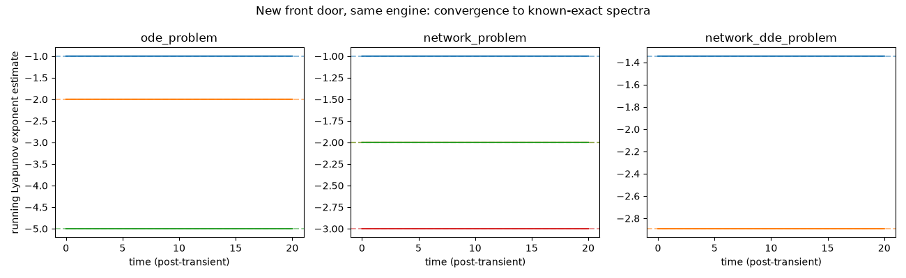
plain ODE
  exact eigenvalues:  [-1. -2. -5.]
  ode_problem estimate: [-1.00000095 -1.99999905 -5.        ]

2. Coupled network: Network + network_problem(..., integrator=...)

Same 4-node cycle network as 04_linear_network.py: identical scalar node dynamics x_i' = gamma*x_i + c_i coupled linearly through adjacency matrix W, so the exact spectrum is eig(gamma*I + G*W). Network names weights/cvar_indices as one object instead of two parallel positional arguments; network_problem reads them off it and, like ode_problem above, folds in state0/dt too.

weights = jnp.array([
    [0., 1., 0., 1.],
    [1., 0., 1., 0.],
    [0., 1., 0., 1.],
    [1., 0., 1., 0.],
])
gamma, G = -2.0, 0.5
expected_net = np.sort(np.linalg.eigvalsh(gamma * np.eye(4) + G * np.array(weights)))[::-1]

model = ModelSpec(
    name="linear_node",
    state_variables=(StateVar("x", default_init=0.0),),
    parameters=(Parameter("gamma", gamma),),
    cvar=("x",),
    dfun_str={"x": "gamma * x + c"},
)
dfun = build_jax_dfun(model)
network = lyapax.Network(weights=weights, cvar_indices=model.cvar_indices)

problem_net = lyapax.network_problem(
    dfun, network, lc.linear_coupling(a=1.0, b=0.0),
    params={"gamma": gamma, "G": G}, state0=jnp.array([0.3, -0.1, 0.2, -0.4]),
    dt=1e-3, integrator="heun",
)
result_net = lyapax.lyapunov_spectrum(
    problem_net, n_steps=20_000, renorm_every=10, t_transient=5.0,
)

print("coupled network")
print(f"  exact eigenvalues:      {expected_net}")
print(f"  network_problem estimate: {np.array(result_net.exponents)}")

coupled network
  exact eigenvalues:      [-1. -2. -2. -3.]
  network_problem estimate: [-1.00000336 -1.99999657 -1.99999842 -2.9999943 ]

3. Delayed coupled network: network_dde_problem

Same 2-node delayed linear network as 08_delayed_coupling.py (x1' = gamma*x1 + G*x2(t-tau), x2' = gamma*x2 + G*x1(t-tau)), whose symmetric/antisymmetric modes have closed-form Lambert-W exponents. There, building this required Connectivity for the delay matrix and a raw (state0, buf0, params, dt) call into lyapunov_spectrum_dde. network_dde_problem collapses that into the same dynamics/network/coupling/integrator recipe as the zero-delay case above, plus tau – the ring buffer (buf0) and its initial constant history are built for you.

weights_2 = jnp.array([[0., 1.], [1., 0.]])
network_2 = lyapax.Network(weights=weights_2, cvar_indices=model.cvar_indices)
tau = 0.2
dt_dde = 1e-3

problem = lyapax.network_dde_problem(
    dfun, network_2, lc.linear_coupling(a=1.0, b=0.0),
    params={"gamma": gamma, "G": G}, state0=jnp.array([[0.3, -0.2]]),
    dt=dt_dde, tau=tau, integrator="heun",
)
result_dde = lyapax.lyapunov_spectrum_dde(
    problem, n_steps=20_000, k=2, renorm_every=10, t_transient=5.0,
)


def lambda_sym(tau):
    return gamma + float((lambertw(G * tau * np.exp(-gamma * tau), k=0) / tau).real)


def lambda_antisym(tau):
    return gamma + float((lambertw(-G * tau * np.exp(-gamma * tau), k=0) / tau).real)


expected_dde = np.array([lambda_sym(tau), lambda_antisym(tau)])
print("delayed coupled network")
print(f"  exact (Lambert W):            {expected_dde}")
print(f"  network_dde_problem estimate: {np.array(result_dde.exponents)}")

delayed coupled network
  exact (Lambert W):            [-1.34559461 -2.89150289]
  network_dde_problem estimate: [-1.34520443 -2.89307176]

All three estimates converging to their known-exact answers, side by side.

fig, axes = plt.subplots(1, 3, figsize=(13, 4), sharey=False)

for ax, result, expected, title in zip(
    axes,
    [result_ode, result_net, result_dde],
    [expected_ode, expected_net, expected_dde],
    ["ode_problem", "network_problem", "network_dde_problem"],
):
    h, t = np.array(result.history), np.array(result.times)
    for i, lam in enumerate(expected):
        ax.plot(t, h[:, i], color=f"C{i}")
        ax.axhline(lam, color=f"C{i}", linestyle="--", alpha=0.5)
    ax.set_xlabel("time (post-transient)")
    ax.set_title(title)
axes[0].set_ylabel("running Lyapunov exponent estimate")
fig.suptitle("New front door, same engine: convergence to known-exact spectra")
fig.tight_layout()
plt.show()