Kaplan-Yorke (Lyapunov) dimension

The Kaplan-Yorke dimension (Kaplan & Yorke, 1979) estimates a chaotic attractor’s fractal dimension directly from its Lyapunov spectrum, with no extra simulation: sort the exponents descending, walk the cumulative sum lambda_1, lambda_1 + lambda_2, ... until it would go negative, and interpolate the fractional part from where it crosses zero. It’s a standard companion metric to a Lyapunov spectrum – pure post-processing of LyapunovResult.exponents, exposed here as lyapax.core.kaplan_yorke_dimension.

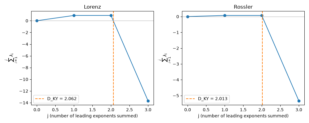
This demo computes the full spectrum for Lorenz and Rossler, reads off the Kaplan-Yorke dimension for each, and plots the cumulative-sum curve so the “where does it cross zero” mechanics behind the formula are visible directly, rather than just printing a number.

import os

os.environ["JAX_PLATFORMS"] = "cpu"

import jax
import jax.numpy as jnp
import matplotlib.pyplot as plt
import numpy as np

jax.config.update("jax_enable_x64", True)

from lyapax import systems
from lyapax.core import kaplan_yorke_dimension, lyapunov_spectrum, ode_problem

dt = 1e-2

rhs_lorenz = systems.lorenz(sigma=10.0, rho=28.0, beta=8.0 / 3.0)
problem_lorenz = ode_problem(rhs_lorenz, state0=jnp.array([1.0, 1.0, 1.0]), dt=dt)
result_lorenz = lyapunov_spectrum(
    problem_lorenz, n_steps=50_000, renorm_every=10, t_transient=100.0)

rhs_rossler = systems.rossler(a=0.2, b=0.2, c=5.7)
problem_rossler = ode_problem(rhs_rossler, state0=jnp.array([1.0, 1.0, 1.0]), dt=dt)
result_rossler = lyapunov_spectrum(
    problem_rossler, n_steps=200_000, renorm_every=10, t_transient=200.0)

systems_ = [("Lorenz", result_lorenz, 2.06), ("Rossler", result_rossler, 2.01)]

for name, result, published in systems_:
    exponents = np.array(result.exponents)
    ky = kaplan_yorke_dimension(exponents)
    print(f"{name}: lambda = {exponents}")
    print(f"  Kaplan-Yorke dimension = {ky:.4f}   (published ~{published})")

Lorenz: lambda = [ 9.01718228e-01  1.66890342e-03 -1.45699518e+01]
  Kaplan-Yorke dimension = 2.0620   (published ~2.06)
Rossler: lambda = [ 7.07982131e-02 -1.24925864e-04 -5.39916724e+00]
  Kaplan-Yorke dimension = 2.0131   (published ~2.01)

fig, axes = plt.subplots(1, 2, figsize=(10, 4))
for ax, (name, result, _) in zip(axes, systems_):
    exponents = np.array(result.exponents)
    cumsum = np.concatenate([[0.0], np.cumsum(exponents)])
    ax.plot(range(len(cumsum)), cumsum, marker="o")
    ax.axhline(0.0, color="gray", lw=0.5)
    ky = kaplan_yorke_dimension(exponents)
    ax.axvline(ky, color="C1", linestyle="--", label=f"D_KY = {ky:.3f}")
    ax.set_xlabel("j (number of leading exponents summed)")
    ax.set_ylabel(r"$\sum_{i=1}^{j} \lambda_i$")
    ax.set_title(name)
    ax.legend()
fig.tight_layout()
plt.show()

A partial spectrum (k < d) can only give the Kaplan-Yorke dimension if the cumulative sum actually crosses zero within the tracked exponents. Passing d_total makes that assumption explicit: if the crossing point turns out to lie beyond what was tracked, kaplan_yorke_dimension raises instead of silently understating the dimension as len(exponents).

try:
    kaplan_yorke_dimension(jnp.array([0.9, 0.5]), d_total=3)
except ValueError as exc:
    print(f"\npartial-spectrum guard triggered as expected:\n  {exc}")

partial-spectrum guard triggered as expected:
  kaplan_yorke_dimension: the cumulative sum of all 2 tracked exponents never goes negative, so the Kaplan-Yorke crossing point lies beyond the tracked partial spectrum (d_total=3 > k=2) -- track more exponents (a larger k) to find it. Omit d_total only when `exponents` is already the full spectrum.