Matrix-free tangent propagation: dense jacfwd vs jvp/vmap

Tracking only the top k Lyapunov exponents of a d-dimensional system (k < d) should only cost O(k) work per step, not O(d) – that’s the whole point of a partial spectrum. The naive way to linearize a step function, jax.jacfwd(step_fn)(state), doesn’t get this for free: it always computes the full d x d Jacobian and only afterwards multiplies by the k tracked tangent columns (jac @ Y), so the d - k untracked columns are wasted work. lyapax.core.lyapunov_spectrum instead computes exactly the k columns that are actually needed, via one jax.jvp (forward-mode directional derivative) per tracked column, batched together with jax.vmap – the same “matrix-free” idea underlying lyapax.dde.lyapunov_spectrum_dde’s delayed-network engine, here applied to the plain (non-delayed) case. See tests/test_lyapunov_core.py::test_tangent_propagation_matches_dense_jacfwd for the correctness check (this script is purely about cost).

The comparison. A Kuramoto network (same construction as 05_kuramoto_sync.py and 09_kuramoto_delayed_network.py) at growing size d (= n_nodes, one phase per node), tracking a fixed small k=5. 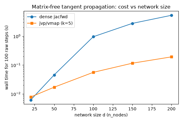Both a hand-rolled dense-jacfwd step and the library’s actual jvp/vmap step (the same code lyapax.core.lyapunov_spectrum runs internally) are JIT-compiled and timed after a warmup call, so this measures steady-state per-step cost, not one-time tracing/compilation overhead. Dense cost should grow much faster than jvp/vmap cost as d grows, since k (what jvp/vmap actually pays for) stays fixed while dense keeps paying for all d columns regardless.

import os

os.environ["JAX_PLATFORMS"] = "cpu"
import time

import jax
import jax.numpy as jnp
import matplotlib.pyplot as plt
import numpy as np

jax.config.update("jax_enable_x64", True)

from lyapax.core import lyapunov_spectrum
from lyapax.coupling import kuramoto_coupling
from lyapax.network import Network, network_problem
from lyapax.simulator import ModelSpec, Parameter, StateVar, build_jax_dfun

def make_kuramoto_problem(n_nodes, dt):
    weights = jnp.ones((n_nodes, n_nodes)) - jnp.eye(n_nodes)
    model = ModelSpec(
        name="kuramoto", state_variables=(StateVar("theta", default_init=0.0),),
        parameters=(Parameter("omega", 0.0),), cvar=("theta",),
        dfun_str={"theta": "omega + c"},
    )
    dfun = build_jax_dfun(model)
    params = {"omega": jnp.linspace(-1.0, 1.0, n_nodes), "G": 1.0}
    network = Network(weights=weights, cvar_indices=model.cvar_indices)
    state0 = jnp.linspace(0.0, 2 * jnp.pi, n_nodes, endpoint=False)
    return network_problem(
        dfun, network, kuramoto_coupling(alpha=0.0),
        params=params, state0=state0, dt=dt,
    )

dt = 1e-2
k = 5
node_sizes = [20, 50, 100, 150, 200]
n_raw_steps = 100
dense_times, jvp_times = [], []

for n_nodes in node_sizes:
    problem = make_kuramoto_problem(n_nodes, dt)
    step, state0 = problem.step_fn, problem.state0
    d = state0.shape[0]
    key = jax.random.PRNGKey(0)
    Y0, _ = jnp.linalg.qr(jax.random.normal(key, (d, k), dtype=jnp.float64))

    @jax.jit
    def dense_step(state, Y):
        jac = jax.jacfwd(step)(state)
        return step(state), jac @ Y

    @jax.jit
    def jvp_step(state, Y):
        def _single_column(y_col):
            return jax.jvp(step, (state,), (y_col,))
        new_state_rep, new_Y = jax.vmap(
            _single_column, in_axes=-1, out_axes=(0, -1))(Y)
        return new_state_rep[0], new_Y

    # Warmup: pay JIT tracing/compilation once, outside the timed loop.
    s, Y = dense_step(state0, Y0)
    jax.block_until_ready((s, Y))
    s, Y = jvp_step(state0, Y0)
    jax.block_until_ready((s, Y))

    t0 = time.perf_counter()
    s, Y = state0, Y0
    for _ in range(n_raw_steps):
        s, Y = dense_step(s, Y)
    jax.block_until_ready((s, Y))
    t_dense = time.perf_counter() - t0

    t0 = time.perf_counter()
    s, Y = state0, Y0
    for _ in range(n_raw_steps):
        s, Y = jvp_step(s, Y)
    jax.block_until_ready((s, Y))
    t_jvp = time.perf_counter() - t0

    dense_times.append(t_dense)
    jvp_times.append(t_jvp)
    print(f"d={d:4d}  dense jacfwd={t_dense:6.3f}s  jvp/vmap={t_jvp:6.3f}s  "
          f"speedup={t_dense / t_jvp:5.1f}x")

d=  20  dense jacfwd= 0.006s  jvp/vmap= 0.008s  speedup=  0.8x
d=  50  dense jacfwd= 0.046s  jvp/vmap= 0.017s  speedup=  2.7x
d= 100  dense jacfwd= 0.957s  jvp/vmap= 0.056s  speedup= 17.1x
d= 150  dense jacfwd= 2.776s  jvp/vmap= 0.116s  speedup= 24.0x
d= 200  dense jacfwd= 5.285s  jvp/vmap= 0.192s  speedup= 27.5x

fig, ax = plt.subplots(figsize=(6, 4))
ax.plot(node_sizes, dense_times, "o-", label="dense jacfwd")
ax.plot(node_sizes, jvp_times, "s-", label=f"jvp/vmap (k={k})")
ax.set_xlabel("network size d (n_nodes)")
ax.set_ylabel(f"wall time for {n_raw_steps} raw steps (s)")
ax.set_yscale("log")
ax.set_title("Matrix-free tangent propagation: cost vs network size")
ax.legend()
fig.tight_layout()
plt.show()

— confirm lyapunov_spectrum itself (now jvp/vmap-based) scales to a full accumulation run on the largest network above, not just the raw per-step timing loop –

problem = make_kuramoto_problem(200, dt)
t0 = time.perf_counter()
result = lyapunov_spectrum(
    problem, n_steps=2_000, k=5, renorm_every=10, t_transient=5.0,
)
elapsed = time.perf_counter() - t0
print(f"\nlyapunov_spectrum, d=200, k=5, 2000 steps: {elapsed:.2f}s")
print(f"top-5 exponents: {np.array(result.exponents)}")

lyapunov_spectrum, d=200, k=5, 2000 steps: 1.84s
top-5 exponents: [0.032741   0.03237385 0.02422666 0.01651107 0.01513247]