Convergence diagnostics: convergence_drift + resume

lyapunov_spectrum always runs a fixed n_steps – there is no built-in stopping criterion, adaptive or otherwise (see 01_linear_ode.py and every other example: they all pick n_steps up front and never revisit it). Two pieces turn that into a “run a chunk, look, continue if not converged” workflow:

• lyapax.core.convergence_drift(result, tol=...) compares the final running estimate in result.history to the estimate from a fraction of the run ago, and flags each exponent converged/not-converged.

• result.checkpoint / lyapunov_spectrum(..., resume=...) lets the next call continue this run – same trajectory point, same tangent basis, no re-transient – instead of restarting from scratch. Its history/times continue the same cumulative running estimate, so concatenating each chunk’s history gives one continuous curve.

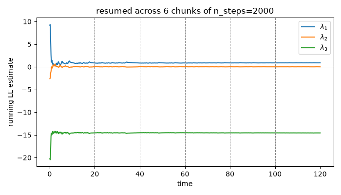
Reading the plot. Each vertical dashed line is a resume point (one lyapunov_spectrum call ending, the next picking up from its checkpoint); the curve is seamless across them, and the loop below stops as soon as convergence_drift reports lambda1 has settled.

import os

os.environ["JAX_PLATFORMS"] = "cpu"

import jax
import jax.numpy as jnp
import matplotlib.pyplot as plt
import numpy as np

jax.config.update("jax_enable_x64", True)
# QR and reduction ops are not bitwise-identical across backends, so the
# chunk where a tight convergence_drift(tol=...) first passes can shift
# between CPU and GPU -- report the backend alongside the result.
print(f"JAX backend: {jax.default_backend()}")

from lyapax import lyapunov_spectrum, ode_problem, systems
from lyapax.core import convergence_drift

JAX backend: cpu

rhs = systems.lorenz(sigma=10.0, rho=28.0, beta=8.0 / 3.0)
problem = ode_problem(rhs, state0=jnp.array([1.0, 1.0, 1.0]), dt=1e-2)
chunk, tol = 2_000, 1e-2

result = lyapunov_spectrum(problem, n_steps=chunk, renorm_every=10, t_transient=100.0)
history_chunks, time_chunks = [np.array(result.history)], [np.array(result.times)]
drift = convergence_drift(result, tol=tol)
print(f"chunk 1: lambda1={float(result.exponents[0]):.4f}  converged={bool(drift.converged[0])}")

while not bool(drift.converged[0]):
    result = lyapunov_spectrum(problem, n_steps=chunk, renorm_every=10, resume=result.checkpoint)
    history_chunks.append(np.array(result.history))
    time_chunks.append(np.array(result.times))
    drift = convergence_drift(result, tol=tol)
    print(f"chunk {len(history_chunks)}: lambda1={float(result.exponents[0]):.4f}  "
          f"converged={bool(drift.converged[0])}")

chunk 1: lambda1=0.8367  converged=False
chunk 2: lambda1=0.8415  converged=False
chunk 3: lambda1=0.8770  converged=False
chunk 4: lambda1=0.8674  converged=False
chunk 5: lambda1=0.8972  converged=False
chunk 6: lambda1=0.8911  converged=True

history, times = np.concatenate(history_chunks), np.concatenate(time_chunks)

fig, ax = plt.subplots(figsize=(7, 4))
for i in range(3):
    ax.plot(times, history[:, i], label=rf"$\lambda_{i + 1}$")
for c in time_chunks[:-1]:
    ax.axvline(c[-1], color="gray", linestyle="--", linewidth=0.8)
ax.axhline(0.0, color="gray", lw=0.5)
ax.set_xlabel("time")
ax.set_ylabel("running LE estimate")
ax.set_title(f"resumed across {len(history_chunks)} chunks of n_steps={chunk}")
ax.legend()
fig.tight_layout()
plt.show()