Benchmarks

How lyapax’s Lyapunov-exponent estimates and wall-clock performance compare against other tools that compute the same quantity, on the same benchmark systems lyapax’s own test suite is validated against (see Validation: how lyapax’s results are checked).

The tables on this page are generated, not hand-written, and are refreshed periodically rather than on every commit or doc build - treat any specific number below as a snapshot, not a live guarantee. To reproduce or refresh them yourself:

python benchmarks/collect_results.py   # runs every tool, writes benchmarks/results.json
python benchmarks/report_tables.py --write   # regenerates the tables below from that file

collect_results.py needs optional dependencies this doc build doesn’t carry (a Julia install with ChaosTools.jl, jitcode/jitcdde, and, for the GPU column, an actual GPU) - see benchmarks/collect_results.py’s module docstring for the full requirements. That’s also why these tables are committed as a static snapshot (benchmarks/results.json) instead of being executed as part of building this documentation.

Comparison targets

• jitcode - the established Python reference for ODE Lyapunov spectra (symbolic → compiled C).

• jitcdde - the DDE counterpart, and the closest existing precedent for lyapax’s own delayed-system engine.

• ChaosTools.jl

  • the most widely used dynamical-systems toolbox in Julia; covers both continuous and discrete (map) systems.

• Published/analytic references - exact eigenvalues, Lambert-W roots, or literature values, wherever a benchmark system has one.

None of these share lyapax’s exact integration scheme or default tolerances, so this is a cross-validation of the computed exponents against independent implementations, not a claim that every tool is configured identically. Step size, transient length, total run length, and QR-renormalization interval are matched as closely as each tool’s API allows; where a tool’s own defaults differ meaningfully (e.g. adaptive step control), that’s left as-is rather than silently normalized away.

Accuracy

Each row compares the estimated Lyapunov exponent(s) (or, for chaotic systems without a closed-form spectrum, a structural invariant like sum(λ)) against an exact or published reference, across whichever tools support that system class (map-only systems have no jitcode column since it’s ODE-only; DDE systems have no ChaosTools.jl column since it has no delay-equation support).

ODE systems

System	lyapax	lyapax (RK6)	jitcode	ChaosTools.jl	ChaosTools.jl (RK4)	ChaosTools.jl (Vern6)	Reference	Notes
Linear ODE (Tier 0.1)	[-1.0000, -2.0000, -5.0000]	[-1.0000, -2.0000, -5.0000]	[-1.0000, -2.0000, -5.0000]	[-1.0000, -2.0000, -5.0000]	[-1.0000, -2.0000, -5.0000]	[-1.0000, -2.0000, -5.0000]	exact [-1, -2, -5]	max abs diff from reference – lyapax: 9.45e-07, lyapax (RK6): 9.45e-07, jitcode: 3.91e-05, ChaosTools.jl: 8.76e-11, ChaosTools.jl (RK4): 2.80e-11, ChaosTools.jl (Vern6): 2.03e-12
Lorenz λ1 (Tier 1.1/2)	0.90172	0.90878	0.91444	0.89674	0.90632	0.91334	published ≈0.9056	max abs diff from reference – lyapax: 3.88e-03, lyapax (RK6): 3.18e-03, jitcode: 8.84e-03, ChaosTools.jl: 8.86e-03, ChaosTools.jl (RK4): 7.17e-04, ChaosTools.jl (Vern6): 7.74e-03
Lorenz sum(λ)	-13.6666	-13.6667	-13.6667	-13.5228	-13.6666	-13.6667	exact -13.6667 (-(σ+1+β))	max abs diff from reference – lyapax: 1.02e-04, lyapax (RK6): 1.79e-09, jitcode: 1.53e-06, ChaosTools.jl: 1.44e-01, ChaosTools.jl (RK4): 1.03e-04, ChaosTools.jl (Vern6): 1.82e-09
Rössler λ1 (Tier 1.2/2)	0.07080	0.08017	0.07011	0.06205	0.07545	0.07264	qualitative ≈0.07	max abs diff from reference – lyapax: 7.98e-04, lyapax (RK6): 1.02e-02, jitcode: 1.08e-04, ChaosTools.jl: 7.95e-03, ChaosTools.jl (RK4): 5.45e-03, ChaosTools.jl (Vern6): 2.64e-03
4-node linear network (Tier 3.1)	[-1.0000, -2.0000, -2.0000, -3.0000]	[-1.0000, -2.0000, -2.0000, -3.0000]	[-1.0000, -2.0000, -2.0000, -3.0000]	[-1.0000, -2.0000, -2.0000, -3.0000]	[-1.0000, -2.0000, -2.0000, -3.0000]	[-1.0000, -2.0000, -2.0000, -3.0000]	exact [-1, -2, -2, -3]	max abs diff from reference – lyapax: 3.53e-06, lyapax (RK6): 3.53e-06, jitcode: 1.09e-05, ChaosTools.jl: 2.23e-06, ChaosTools.jl (RK4): 2.18e-06, ChaosTools.jl (Vern6): 2.18e-06

Map systems

System	lyapax	ChaosTools.jl	Exact	Notes
Logistic map r=4 (Tier 0.2)	0.6931520	0.6931520	ln 2 = 0.6931472	max abs diff from reference – lyapax: 4.84e-06, ChaosTools.jl: 4.84e-06
Tent map (Tier 0.2)	0.6931472	0.6931472	ln 2 = 0.6931472	max abs diff from reference – lyapax: 1.11e-16, ChaosTools.jl: 3.97e-13
Hénon map, sum(λ) (Tier 0.3)	-1.203973	-1.203973	ln 0.3 = -1.203973	max abs diff from reference – lyapax: 2.22e-16, ChaosTools.jl: 2.04e-14; individual exponents: lyapax [0.4193, -1.6233]; ChaosTools.jl [0.4191, -1.6231]

DDE systems

System	lyapax	lyapax (RK6)	jitcdde	Reference	Notes
Linear scalar DDE (Tier 4.2)	-0.60050	-0.60050	-0.59830	Lambert W root -0.598304	max abs diff from reference – lyapax: 2.19e-03, lyapax (RK6): 2.19e-03, jitcdde: 7.26e-07
Mackey-Glass λ1 (Tier 4.1)	0.00796	0.00727	0.00517	qualitative 1e-03-1e-02	lyapax inside band; lyapax (RK6) inside band; jitcdde inside band
Mackey-Glass KY dimension	2.206	2.191	2.133	2.0-3.0	lyapax inside band; lyapax (RK6) inside band; jitcdde inside band
2-node delayed linear network (Tier 4.3)	not yet run	not yet run	not yet run	Lambert W root (2x2)	deferred – not yet run against jitcdde

Performance

Steady-state per-call wall-clock time (each tool’s JIT/compile step has already run by the time these numbers are measured). The GPU columns re-run the same lyapax scripts with a CUDA backend rather than CPU - see benchmarks/collect_results.py for how that pass is skipped (with a warning, not a failure) when no working GPU is found.

The default ChaosTools.jl column uses its own idiomatic choice (Tsit5, adaptive step control) - a different algorithm from lyapax’s fixed-step rk4/rk6, so that timing isn’t a same-method comparison (see the “Comparison targets” fairness note above). The ChaosTools.jl (RK4) and ChaosTools.jl (Vern6) columns close that gap: they run OrdinaryDiffEq.jl’s RK4() and Vern6() (the exact tableau lyapax’s rk6_step implements - see lyapax.integrators.rk6_combine’s docstring) with adaptive=false at lyapax’s own fixed dt, so the two sides are running the literal same algorithm and step size. The gap that remains at that point is a genuine implementation/runtime difference (Julia/LLVM vs. JAX/XLA at these small state sizes), not an algorithm mismatch.

System	lyapax	lyapax (RK6)	lyapax (GPU)	lyapax (RK6, GPU)	jitcode	jitcdde	ChaosTools.jl	ChaosTools.jl (RK4)	ChaosTools.jl (Vern6)
Linear ODE (Tier 0.1)	0.270s	0.396s	0.961s	1.488s	0.194s	–	0.003s	0.007s	0.010s
Lorenz	0.406s	0.676s	1.834s	3.448s	0.660s	–	0.010s	0.022s	0.040s
Rössler	0.420s	0.735s	4.727s	9.369s	2.076s	–	0.032s	0.074s	0.116s
4-node network (Tier 3.1)	0.434s	0.749s	1.208s	2.268s	0.195s	–	0.004s	0.012s	0.046s
Linear scalar DDE (Tier 4.2)	0.327s	0.422s	0.700s	0.848s	–	0.017s	–	–	–
Mackey-Glass	0.615s	0.915s	1.399s	1.984s	–	10.502s	–	–	–

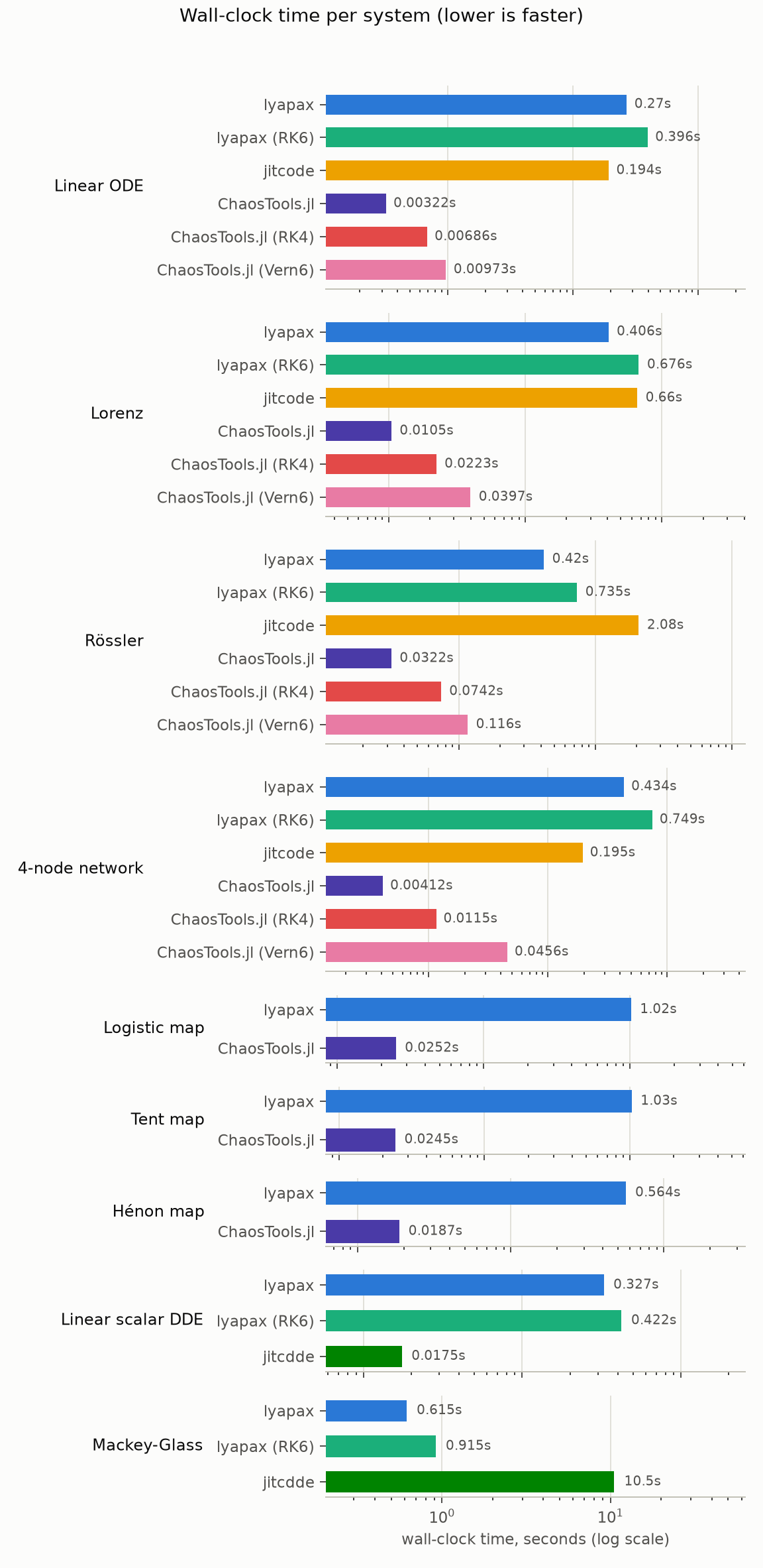
The plot below is generated from the same benchmarks/results.json snapshot as the tables above; regenerate it with python benchmarks/report_plots.py. It’s every tool’s steady-state wall-clock time per system, log-scaled since the range spans several orders of magnitude – jitcode/jitcdde are the tools closest to lyapax’s own execution model (a one-time trace/compile, then a tight numerical loop for every call after); ChaosTools.jl has near-zero per-call overhead on these small toy systems and is the fastest tool for most of them regardless.

Network-size scaling

Every system above is small (3–4 state dimensions) - deliberately, so each has an exact or published reference to validate against. But it also means none of them exercise the part of lyapax’s design meant for bigger problems. This section uses one further system, a dense (all-to-all) Kuramoto network, at increasing size d, tracking a fixed k=5 partial spectrum - the same system as 10_matrix_free_scaling.py / 14_gpu_acceleration.py, run here across tools instead of just lyapax CPU vs. GPU. It’s a performance-only comparison - a short, no-transient run, not validated against a reference spectrum the way the tables above are - so read the timings, not the exponent values.

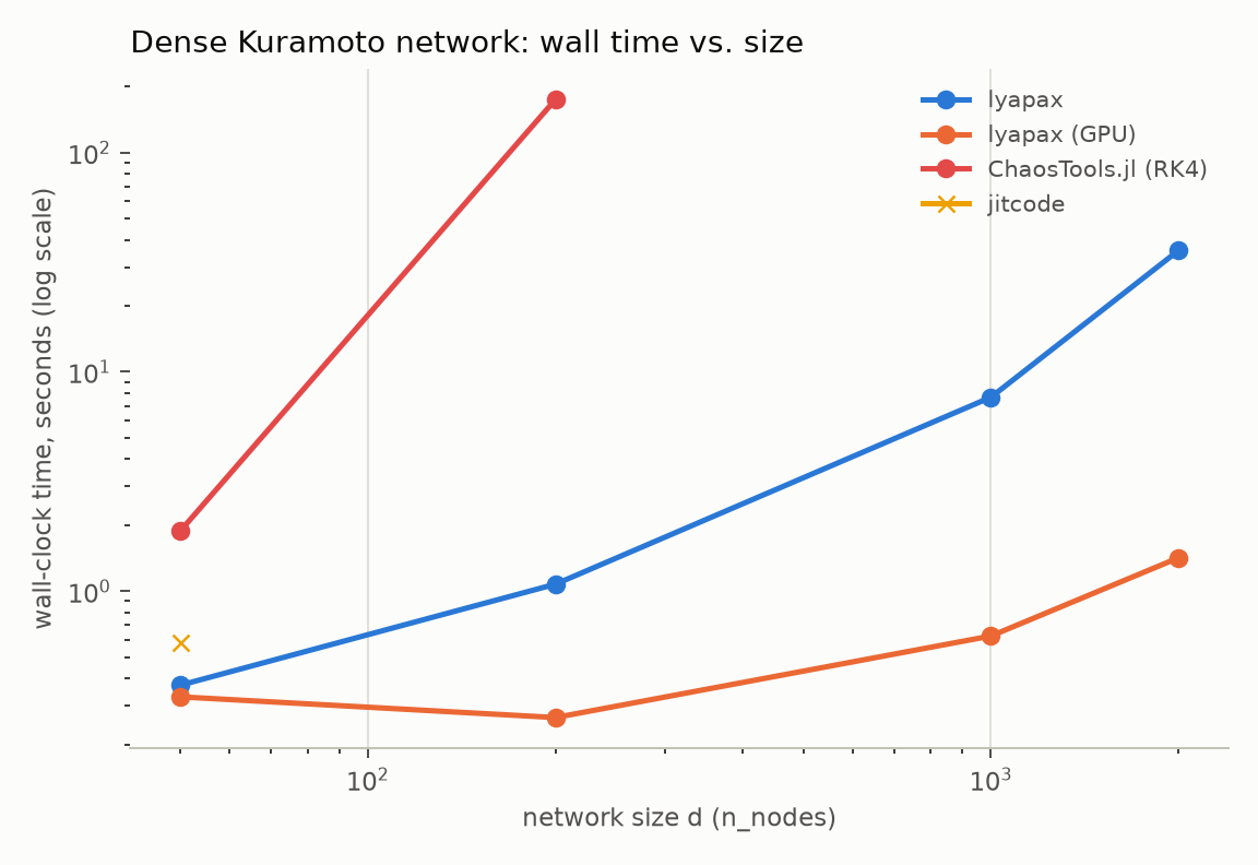
lyapax’s cost here is dominated by k, not d. jax.jvp computes only the k=5 tangent directions actually requested, regardless of how large the network is (see lyapax.core.lyapunov_spectrum’s docstring). That’s why ChaosTools.jl and jitcode - both of which stop well short of lyapax’s full d=50/200/1000/2000 sweep - aren’t a same-algorithm comparison being run partway; they’re at (or past) their own scaling limit:

• ChaosTools.jl stops at d=200 (using the fixed-step RK4() established above as the fair algorithm to compare). Its tangent propagation forms the full dense d x d Jacobian via ForwardDiff every step, regardless of k - the opposite of lyapax’s matrix-free approach. The table below shows this cost growing far worse than quadratically between d=50 and d=200; a direct test at d=1000 was abandoned after running well past ten minutes without finishing a single call. This is a genuine per-call cost, not a one-time compile tax - a direct comparison of that same d=200 run’s first and warm calls came out within a few percent of each other, unlike a case dominated by JIT/compile overhead.

• jitcode stops at d=50 for a different reason: it differentiates the right-hand side symbolically before compiling to C, and that compile step alone took on the order of a minute for a dense d=50 network (~2,450 nonzero coupling terms) in a direct test, before a single integration step ran - a cost the table below doesn’t show, since it (like the rest of this page) reports steady-state, post-compile time only. Unlike ChaosTools.jl’s bottleneck, this one is front-loaded - once compiled, jitcode’s own steady-state call is fast - but the compile cost itself scales with network density and would only be worse at d=200+.

lyapax pays neither cost at any of these sizes: no symbolic differentiation step to compile, and no dense Jacobian to form at run time.

Network size (d)	lyapax	lyapax (GPU)	ChaosTools.jl (RK4)	jitcode
50	0.372s	0.330s	1.878s	0.585s
200	1.075s	0.265s	174.227s	not attempted
1000	7.659s	0.624s	not attempted	not attempted
2000	35.773s	1.419s	not attempted	not attempted

The d=1000/d=2000 rows are also where lyapax’s GPU backend earns its keep - unlike the small 3–4-dimensional systems above, where GPU lost outright to CPU (see the performance table’s GPU columns), a dense d=2000 network’s per-step arithmetic is large enough to amortize GPU dispatch overhead.