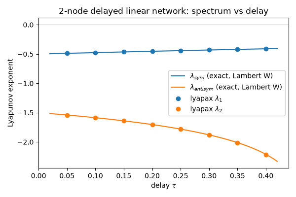
Delayed coupling: two-node linear DDE network vs delay

The simplest possible “delayed coupling” demo: two identical linear nodes coupled through each other’s delayed state, x1' = gamma*x1 + G*x2(t-tau), x2' = gamma*x2 + G*x1(t-tau). This sweeps the delay tau itself, to show what delayed coupling does to the spectrum – how it differs from the zero-delay case in 04_linear_network.py.

Why this system. Its characteristic equation is tractable: the symmetric mode (x1=x2) gives lambda_sym = gamma + W(G*tau*e^{-gamma*tau})/tau and the antisymmetric mode (x1=-x2) gives lambda_antisym = gamma + W(-G*tau*e^{-gamma*tau})/tau (Lambert W, principal branch) – so every point on the sweep below has an independent closed-form answer, not just the single spot-check the test performs.

Delay range, deliberately narrow. The antisymmetric branch’s Lambert-W argument, -G*tau*e^{-gamma*tau}, crosses the branch point at -1/e around tau ~ 0.46 for the parameters below – past that, W’s principal branch stops being real/single-valued and taking .real of it no longer tracks the true dominant root (verified numerically while writing this demo: the naive formula produces a non-monotonic jump right at the crossing, an artifact of the branch point, not real dynamics). The sweep below stays at tau <= 0.4, safely inside the region where the closed form is valid, so every plotted “exact” point is trustworthy.

The machinery. Coupling between two different nodes’ delayed states (as opposed to a single scalar equation delayed against its own past, e.g. Mackey-Glass) needs the general, per-edge delay_steps path: simulator.Connectivity(weights, tract_lengths, speed) turns a physical tau into an integer delay_steps matrix and the ring-buffer horizon needed to store enough history, exactly as lyapax.dde.resolve_tau_steps does for a single scalar delay – then simulator.make_step_fn(..., delay_steps=...) and lyapax.dde.lyapunov_spectrum_dde do the rest: propagate the state and its ring-buffer history together, periodically re-orthonormalizing the tangent directions via QR, the same Benettin’s-method idea as the non-delayed engine, just carrying delay history alongside the state.

Deliberately staying low-level here: network_dde_problem (the problem-object front door used by 09_kuramoto_delayed_network.py and 12_public_api_overview.py) only covers a single uniform delay shared by every edge, and explicitly rejects a per-edge delay_steps matrix like the one this script needs – see that function’s docstring. A per-edge delay matrix combined with a custom coupling_fn isn’t wired up at all yet (only this hardcoded-linear delay_steps path is); this script is the one place that still needs the raw Connectivity/make_step_fn/lyapunov_spectrum_dde call form for that reason, not because it predates the new API.

import os

os.environ["JAX_PLATFORMS"] = "cpu"
import time

import jax
import jax.numpy as jnp
import matplotlib.pyplot as plt
import numpy as np
from scipy.special import lambertw

jax.config.update("jax_enable_x64", True)

from lyapax.dde import constant_history_buf0, lyapunov_spectrum_dde
from lyapax.simulator import (
    Connectivity,
    ModelSpec,
    Parameter,
    StateVar,
    build_jax_dfun,
    make_step_fn,
)

gamma, G, dt = -1.0, 0.5, 1e-3


def lambda_sym(tau):
    return gamma + float((lambertw(G * tau * np.exp(-gamma * tau), k=0) / tau).real)


def lambda_antisym(tau):
    return gamma + float((lambertw(-G * tau * np.exp(-gamma * tau), k=0) / tau).real)


model = ModelSpec(
    name="linear_node",
    state_variables=(StateVar("x", default_init=0.0),),
    parameters=(Parameter("gamma", gamma),),
    cvar=("x",),
    dfun_str={"x": "gamma * x + c"},
)
dfun = build_jax_dfun(model)
weights = jnp.array([[0., 1.], [1., 0.]])
params = {"gamma": gamma, "G": G}

tau_values = np.linspace(0.05, 0.4, 8)
lambda1, lambda2 = [], []

t0 = time.perf_counter()
for tau in tau_values:
    conn = Connectivity(
        weights=np.array([[0., 1.], [1., 0.]]),
        tract_lengths=np.array([[0., tau], [tau, 0.]]), speed=1.0,
    )
    delay_steps = jnp.array(conn.delay_steps(dt))
    horizon = conn.horizon(dt)
    step_fn = make_step_fn(
        dfun=dfun, weights=weights, has_delays=True, horizon=horizon, n_nodes=2,
        cvar_indices=model.cvar_indices, dt=dt, delay_steps=delay_steps,
        G_default=G, coup_a=1.0, coup_b=0.0, integrator="heun",
    )
    state0 = jnp.array([[0.3, -0.2]])
    buf0 = constant_history_buf0(state0, horizon)
    result = lyapunov_spectrum_dde(
        step_fn, state0=state0, buf0=buf0, params=params, dt=dt,
        n_steps=20_000, k=2, renorm_every=10, t_transient=5.0,
    )
    lambda1.append(float(result.exponents[0]))
    lambda2.append(float(result.exponents[1]))
elapsed = time.perf_counter() - t0
print(f"swept {len(tau_values)} values of tau in {elapsed:.1f}s "
      f"({elapsed / len(tau_values):.2f}s/run)")
for tau, l1, l2 in zip(tau_values, lambda1, lambda2):
    print(f"  tau={tau:.3f}  lambda1={l1:+.4f} (sym exact {lambda_sym(tau):+.4f})  "
          f"lambda2={l2:+.4f} (antisym exact {lambda_antisym(tau):+.4f})")

swept 8 values of tau in 10.3s (1.28s/run)
  tau=0.050  lambda1=-0.4875 (sym exact -0.4877)  lambda2=-1.5404 (antisym exact -1.5400)
  tau=0.100  lambda1=-0.4755 (sym exact -0.4756)  lambda2=-1.5864 (antisym exact -1.5859)
  tau=0.150  lambda1=-0.4638 (sym exact -0.4640)  lambda2=-1.6400 (antisym exact -1.6394)
  tau=0.200  lambda1=-0.4525 (sym exact -0.4526)  lambda2=-1.7036 (antisym exact -1.7029)
  tau=0.250  lambda1=-0.4415 (sym exact -0.4416)  lambda2=-1.7812 (antisym exact -1.7803)
  tau=0.300  lambda1=-0.4309 (sym exact -0.4310)  lambda2=-1.8796 (antisym exact -1.8784)
  tau=0.350  lambda1=-0.4206 (sym exact -0.4207)  lambda2=-2.0122 (antisym exact -2.0106)
  tau=0.400  lambda1=-0.4106 (sym exact -0.4107)  lambda2=-2.2131 (antisym exact -2.2105)

tau_dense = np.linspace(0.02, 0.42, 200)
sym_dense = [lambda_sym(t) for t in tau_dense]
antisym_dense = [lambda_antisym(t) for t in tau_dense]

fig, ax = plt.subplots(figsize=(6, 4))
ax.plot(tau_dense, sym_dense, "-", color="C0", label=r"$\lambda_{sym}$ (exact, Lambert W)")
ax.plot(tau_dense, antisym_dense, "-", color="C1", label=r"$\lambda_{antisym}$ (exact, Lambert W)")
ax.plot(tau_values, lambda1, "o", color="C0", label=r"lyapax $\lambda_1$")
ax.plot(tau_values, lambda2, "o", color="C1", label=r"lyapax $\lambda_2$")
ax.axhline(0.0, color="gray", lw=0.5)
ax.set_xlabel(r"delay $\tau$")
ax.set_ylabel("Lyapunov exponent")
ax.set_title("2-node delayed linear network: spectrum vs delay")
ax.legend()
fig.tight_layout()
plt.show()